Korean J Anesthesiol Search

CLOSE


Korean J Anesthesiol > Volume 71(3); 2018 > Article
In and Lee: Survival analysis: Part I — analysis of time-to-event
This article has been corrected. See "Survival analysis: Part I — analysis of time-to-event" in Volume 76 on page 83.

Abstract

Length of time is a variable often encountered during data analysis. Survival analysis provides simple, intuitive results concerning time-to-event for events of interest, which are not confined to death. This review introduces methods of analyzing time-to-event. The Kaplan-Meier survival analysis, log-rank test, and Cox proportional hazards regression modeling method are described with examples of hypothetical data.

Introduction

In a clinical trial or clinical study, an investigational treatment is administered to subjects, and the resulting outcome data are collected and analyzed after a certain period of time. Most statistical analysis methods do not include the length of time as a variable, and analysis is made only on the trial outcomes upon completion of the study period, as specified in the study protocol. However, in cases where the outcome yields different interpretations at different points in time, even over a range of only several hours or minutes, it is advantageous to use a statistical analysis method incorporating time as a variable [1]. Poisson regression and survival analysis are typical statistical analysis approaches that analyze the variable which includes the information of the time [2].
The Korean Journal of Anesthesiology has thus far published several papers using survival analysis for clinical outcomes: a comparison of 90-day survival rate for pressure ulcer development or non-development after surgery under general anesthesia [3], a comparison of postoperative 5-year recurrence rate in patients with breast cancer depending on the type of anesthetic agent used [4], and a comparison of airway intubation success rate and intubation time between two types of video laryngoscopy in difficult intubation cases [5]. It is not hard to consider the application of survival analysis for the data of first two articles, using survival analysis for the intubation time comparison in the third paper is not easy to think. For such topics, the main obstacle to the widespread use of survival analysis is the word “survival,” which leads to the misunderstanding that can only be used for data related to death or failure. However, as is the case with the third paper, survival analysis can be applied not only to data of patients’ death, but also to any data related to an “event of interest” that may or may not occur during the observation period.1) The following are several examples of questions for which survival analysis may be applied:
1) How long does symptom improvement last after an epidural injection? (Time to the recurrence of back pain and recurrence vs. non-recurrence)
2) How long is the duration of the effect of antiemetic prophylaxis given to prevent nausea and vomiting resulting from the use of intravenous patient-controlled opioid analgesia? (Duration of nausea/vomiting prevention and manifestation vs. non-manifestation)
3) How long does it take for postoperative cognitive dysfunction caused by general anesthesia to occur? (Time to the occurrence of cognitive dysfunction and occurrence vs. non-occurrence)
In all three examples, after the treatment (epidural injection, administration of antiemetic prophylaxis, administration of general anesthesia), the subsequent event (recurrence of back pain, manifestation of nausea/vomiting, occurrence of cognitive dysfunction) may or may not occur during the specified observation period, and the patient status (occurrence or non-occurrence) and length of time (observation period) are assigned to each participant as variables.
In cases where only rates of occurrence are compared, without regard to the lapse of time until occurrence, the chi-squared test or Fisher’s exact test are sufficient. Conversely, in cases where the time-to-event of interest is analyzed, if the event of interest has occurred for all participants, Student’s t-test or the Mann-Whitney U test may be used. However, even in such cases, non-occurrence or termination of participation (due to improvement or exacerbation, moving, death, etc.) often cannot be ruled out. Also, the observation period may vary due to a limited study period or different outcome time frames. For these reasons, some of data are subject to incompleteness, and these data should be analyzed using another statistical method or excluded. Survival analysis is necessary to analyze incomplete data by setting the time-to-event as a primary outcome. In summary, survival analysis can be applied in a range of situations in which any event of interest (not just mortality) is analyzed in terms of its occurrence or non-occurrence during a specified observation period [1].
Like other statistical methods, survival analysis can be performed using parametric or non-parametric methods. In anesthesia and pain medicine, non-parametric survival analysis is usually preferred because in most cases the data do not satisfy the prerequisites of parametric survival analysis. In parametric survival analysis, a survival model is constructed by performing regression analysis on the assumption that the outcome variables follow a conventionally known distribution, such as the normal distribution, binomial distribution, or Poisson distribution. Common parametric survival models include the Weibull, exponential, log-logistic, lognormal, and generalized gamma models. Non-parametric survival analysis is most commonly performed using the Kaplan-Meier method or Cox proportional hazards regression modeling. In this paper, only non-parametric survival analysis is examined.

Censored Data

Ideal data for survival analysis are those yielded by cases in which the time of treatment is clearly established and all participants are followed up until they experience the event. However, the observation period may end without occurrence of the event because it may be difficult in practice to study all the participants until the occurrence of the event, and because participants can drop out during the observation period. Post-treatment data unavailable for confirmation of occurrence or non-occurrence during the follow-up period are termed censored data2) and are excluded from analysis as missing values in other statistical analysis methods; in survival analysis, however, they are processed as important data influencing the outcome [6,7].
For example, suppose that a clinical study is conducted to examine the efficacy of a new drug for back pain, in which the treatment and event are epidural injection of the new drug and recurrence of back pain, respectively. If it is impossible to confirm recurrence for various reasons such as a car accident, death caused by other diseases, or unavailability of the data needed to confirm recurrence due to movement to another hospital, such cases should be processed as censored data. In censored data, recurrences prior to the last follow-up can be confirmed, but any recurrence after the termination of follow-up cannot be confirmed. Fig. 1 illustrates details of an imaginary study in which six patients were followed over a period of six weeks. Patient 1 participated in the study from the beginning and developed recurrence of back pain in week 4 in the aftermath of a car accident, and therefore is processed as censored data. This data point provides the effectiveness of new drug for 4-week observation. Patient 2 was enrolled in the study in the fourth week, and no recurrence was observed up to week 6. This case of non-recurrence until the end of the observation period is also processed as censored data, with the 2-week follow-up included in the analysis. Patient 3 was enrolled in the fourth week and developed recurrence in week 5; this is a case of a complete data point, with the 1-week follow-up and recurrence included in the analysis. Patient 4 was enrolled in the second week, but the observation was pre-terminated due to loss to follow-up from week 4 onward, resulting in a two-week observation period. Patient 5 participated in the study from the beginning and developed recurrence in week 6, and therefore yields a complete data point. Patient 6 is a case of censored data due to withdrawal caused by uncovered random allocation in week 4, with the 4-week follow-up included in the analysis. To conclude, data related to the occurrence of the treatment-related event are complete data, coded as “X,” and data without indication of occurrence or with occurrence for reasons other than the treatment are censored data, coded as “C” [8].

Survival Function, Hazard Function

“Survival function” is a key term in survival analysis, along with “censoring” and “event.” The concept of a survival function is essential for the understanding of survival analysis.
The survival function is defined as the probability of the outcome event not occurring up to a specific point in time, including the time point of observation (t), and is denoted by S(t). That is, if the event is “recurrence of back pain,” it is the “probability of not having back pain” up to a specific time. In the survival function (Equation 1),3) t = 0 corresponds to a probability of 1.0 (i.e., 100% survival at the onset), and the point in time with 50% survival probability is the median survival time.
S(t) = P (T > t) = 1  F (t)T: Random variable denoting the time of the event. t: Any specified time point. P (T > t): Probability of not experience the event up to and including time t.F (t): Cumulative distribution function
The ratio of the number of events occurring during the entire study period to the total number of observations is termed the “incidence rate.” For example, if the event is death, mortality is the incidence rate. However, since the incidence may not be constant throughout the study period, it may be necessary to calculate the incidence rate at a specific time (t). First, the incidence rate for the period between a specific time t and the next measurement time t + α can be calculated by dividing the number of events occurring between t and t + α by the total number of observations at time t. By α approaches 0, i.e., by taking the limit as the interval between t and t + α closes to 0, the instantaneous incidence rate at t, which constitutes the hazard, can be calculated.4) The hazard function is a function for calculating the instantaneous incidence rate at any given point in time, and is denoted by h (t) [9].

Survival Analysis Using Kaplan-Meier Curves (Estimates)

In the Kaplan-Meier method, the incidence rate as a function of time is calculated by putting the observations in ascending order of time until occurrence. Analysis of the example data in Fig. 1 with the Kaplan-Meier method should thus start by setting the baseline observation of each participant as time 0 (Fig. 2). After arranging all data points, the incidence rate is calculated at each occurrence of the event, followed by survival curve estimation. With the focus of the Kaplan-Meier method on only two variables, namely the observation period and the occurrence/non-occurrence of the event, other variables possibly influencing the occurrence of the event, such as sex and age in the case of the recurrence of back pain, are excluded from analysis [10].
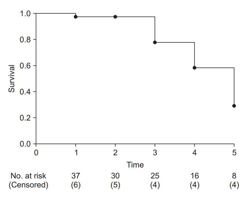
Fig. 3 illustrates the interpretation of the Kaplan-Meier survival curve. Although no standard has yet been established, it is a general practice to show censored data as points or symbols, and decreases in the survival rate (corresponding to the occurrences of the event) as steps. As time points close to the end of study period, the number of participants tend to be decrease abruptly, an incidence rate calculated in this period could not provide clinical significance. So, it is recommended to indicate the number of patients at each calculation point. Some journals set out standards for survival curve creation [11].
Kaplan-Meier survival analysis is used to test for significant differences between survival curves and in median or mean survival time. Therefore, it lends itself well to studies focusing on survival time, i.e., time to the occurrence of the event of interest.

Multiple comparison method for Kaplan-Meier survival analysis

Among the methods for comparing two or more Kaplan-Meier survival curves, such as the Mantel-Haenszel method, log-rank method (Mantel-Cox), Gehan’s generalized Wilcoxon method (Breslow test), and likelihood ratio, the logrank method is most widely used.5) The null hypothesis tested with the log-rank method is that “there is no overall difference between the two survival curves to be compared.” The observed count and the expected count are compared using the chi-square test. The log-rank method is known to have good statistical power when there are considerable differences in the incidence rate among the groups being compared. If three or more groups are compared, pairwise multiple comparisons can also be performed using post-hoc tests such as the Bonferroni test and Holm-Sidak method [12].
Just as the independent t-test should be preceded by testing for normality, the log-rank method is based on several assumptions. The first is the proportional hazards assumption, according to which the hazard ratio (defined in equation 2) should be constant throughout the study period.6) For example, the incidence rate of postoperative nausea/vomiting is highest immediately after surgery and decreases with time, regardless of whether the type of general anesthesia is inhalational or intravenous. That is, the risk of postoperative nausea/vomiting varies (decreases) with time independently of the type of anesthesia. If the proportional hazards assumption is valid, then a finding that the risk of postoperative nausea/vomiting in the patient group receiving an inhalational anesthetic agent is twice that of the patient group receiving an intravenous anesthetic means that there is a twofold difference in hazard at all points in time. With the hazard ratio greater than 1, there is a greater risk of postoperative nausea/vomiting in the inhalational anesthesia group than in the intravenous anesthesia group.7) As illustrated by this example, the hazard ratio offers information that may allow understanding hazard information at a glance [13] (Equation 2).
Hazard ratio =h2(t)h1(t)Where, h1 (t) and h2 (t): hazard functions of groups 1 and 2 t: any specified time point during study period
The proportional hazards assumption and hazard ratio are also important for the Cox proportional regression model, to be explained below [14]. If the proportional hazards assumption is not valid, Gehan’s generalized Wilcoxon test (Breslow test), in which the number of patients exposed to the hazard at the observation point is applied as a weighting factor (instead of 1), or other methods should be used [15].

An example of Kaplan-Meier survival analysis

The results of the survival analysis presented below are derived from imaginary study data on the manifestation/non-manifestation of nausea/vomiting during the first 24 postoperative hours in two groups that received two different antiemetics (Table 1). For convenience of analysis, only age, body weight, and the choice of two of opioid analgesics used intraoperatively are used for analysis. To facilitate understanding, several analytic methods are presented to the same data.
Table 2 outlines the demographic characteristics of the patients included in the study. Although there are not many withdrawals before symptom manifestation in a 24-hour postoperative observational study in actual clinical settings, this virtual study includes a substantial number of dropout patients. Of 104 patients in total, 51 patients (Group A) received antiemetic agent A and 53 patients (Group B) received antiemetic agent B. In Groups A and B, the counts of nausea/vomiting symptoms manifested by the end of 24 postoperative hours are 25 (49.0%) and 38 (71.7%), respectively, and intergroup difference are verified to be statistically significant by the chi-square test (χ2(1) = 5.597, P = 0.018, Cohen’s Φ [phi] = 0.23). The relative risk for Group A compared to Group B is 0.7 (95% CI: 0.5–0.9). Similar results are yielded by incidence rate estimation, although it is an overlapping method, in which the nausea/vomiting symptoms manifested during the first 24 postoperative hours account for 49.0% (95% CI: 35.3–62.7%) of patients in Group A and 71.7% (95% CI: 59.6–83.8%) in Group B, showing a significant intergroup difference (z-test, P = 0.018, Cohen’s h = 0.47). These statistics reflect the results including all censored data without manifestation of nausea/vomiting during the first 24 hours. Given that nausea/vomiting symptoms are potentially observable among the patients with censored data during the study period (24 hours), the accuracy of the above results may not be high. Excluding all censored cases without nausea/vomiting before the first 24 postoperative hours, the number of patients included in the analysis is 73, and the incidence rate recalculated accordingly is 89.3% (95% CI: 77.8–100.0%) for Group A and 84.4% (95% CI: 73.9–95.0%) for Group B. These increased incidence rates reflect the omission of patients who dropped out of the study before completing it (24-hour observation) without manifesting symptoms of nausea/vomiting. Regardless of the researcher’s intention, the actual incidence rates are overestimated due to the omission of patients without symptom manifestation.
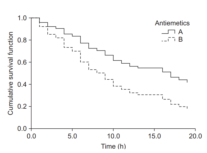
The results of Kaplan-Meier survival analysis for the same datasets are as follows (the observed counts of the event and other results overlapping with those presented above are omitted). The median survival time (length of time free of the target event) is 13.0 hours (25-75%: 8.0–24.0 hours) for Group A and 6.0 hours (25-75%: 3.0-17.0 hours) for Group B; the intergroup difference assessed by the log-rank method is statistically significant (χ2(1) = 6.802, P = 0.009). Examination of the Kaplan-Meier curves for the two groups shows that the cumulative survival rate of Group B rapidly decreases with time compared with that of Group A (Fig. 4).

Cox Proportional Hazards Regression Model

In the Cox proportional hazards regression model, regression analysis is used to process censored data. This method does not presuppose any specific distribution and can analyze any variables that may influence the occurrence, unlike Kaplan-Meier survival analysis, and is thus regarded as a semiparametric method [16,17].
The Cox proportional hazards regression model is based on two assumptions: first, the survival function is an exponential function; second, the hazard ratio for the two compared groups is constant throughout the study period. In other words, the hazard ratio is a constant (HR = λ), and the survival function at any given point in time is expressed as an exponential function of the hazard ratio (s(t) = exp−λt). The null hypothesis for comparison of two survival curves is that “the hazard ratio for the two groups is 1.”
In the Cox proportional hazards regression model, result is derived from the comparison between the risk levels of the occurrence and non-occurrence influenced by a variable which could affect the outcome [18]. The result is an estimate of the hazard ratio of that variable, and is calculated as the corresponding regression coefficient in the regression model. If the hazard ratio of a variable is greater than 1 and poses statistically significance, that variable contributes to increasing the probability of occurrence of the event.
If the hazard ratio of two groups are not maintained at a constant level, a different analysis method should be considered. The Cox proportional hazards regression model cannot be used for analysis in such cases, because a hazard ratio changing with time implies that there may be more than one estimate for the regression coefficient over time. Along with the assumption related to the hazard ratio, basic assumptions required for any sort of regression analysis, such as continuity of variables and absence of interactions between variables, should of course be taken into account [19,20].8)

An example of regression analysis with the Cox proportional hazards regression model

Using the Cox proportional hazards regression model, an analysis was performed on the same example data used above for the Kaplan-Meier survival analysis. As that method is similar to the regression analysis method, the covariates presented in Table 1 are used to estimate the hazard ratio of each covariate and, the corresponding P values are calculated.
Table 3 shows the hazard ratio and P value of each covariate estimated by the analysis using the Cox proportional hazards regression model. These analysis results were obtained by inputting all four covariates into the model, significant hazard ratio was obtained only for the type of antiemetic. The Cox proportional hazards regression model was estimated using the forward conditional method based on the likelihood ratio, and the antiemetics and opioid analgesics used intraoperatively were included in the equation. The hazard ratio for the antiemetics was estimated at 2.0 (95% CI: 1.2–3.3, P = 0.009); antiemetic agent B showed a twofold higher risk of nausea/vomiting during the first 24 postoperative hours compared with antiemetic agent A, and the intraoperative use of fentanyl showed a 4.7-fold risk of postoperative nausea/vomiting compared with remifentanil (hazard ratio 4.7, 95% CI: 2.8–8.1, P < 0.001). The cumulative survival for Group B was found to decrease rapidly (increase in postoperative occurrence of nausea/vomiting) over time when compared with that of Group A (Fig. 5).
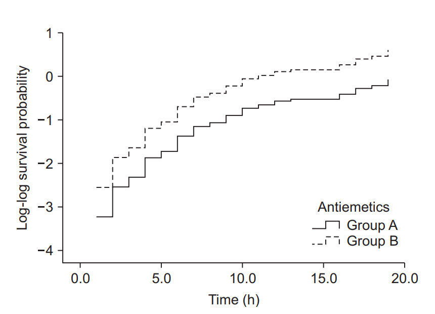
As briefly mentioned above, any estimation based on the Cox proportional hazards regression model must be followed by testing whether the proportional hazards assumption is satisfied. For the example data used here, the log minus log plot (LML plot) is presented as the simplest method for diagnosing problems with the model. The LML plot is a graph constructed by applying the log-log transformation to the survival function. Some statistical program packages optionally output this graph after an analysis based on the Cox proportional hazards regression model, making it possible to easily check compliance with the basic assumption that the hazard ratio is constant throughout the study period. This method for checking compliance with the proportional hazards assumption is essential when using the two survival analysis methods presented in this study, in that a quick intuitive verification is possible by examining the graph, in which the logarithm of the time and the logarithm of the negative logarithm of the estimated survival function are plotted on the x and y axes, respectively. If the LML plots for the comparison groups run parallel to each other without intersecting or meeting, the proportional hazards assumption can be considered valid [21].
Fig. 6 shows the LML plot for the example data. The two curves representing the two antiemetic groups run parallel without meeting or intersecting, demonstrating that the hazard ratios of the two groups with respect to the postoperative nausea/vomiting symptom manifestation are constant over time. In case of a violation of this assumption, which is indicative of the inaccuracy of the Cox proportional hazards regression model, it is desirable to use other methods allowing analysis of time-dependent influences, such as time-dependent Cox regression analysis (non-proportional hazards model).

Sample Size for Survival Analysis

Survival analysis is an analysis method that analyzes the time to an event of interest. In the log-rank test or Cox proportional hazards regression model, the hazard ratio is used for sample size calculation [22]. Just as a normal distribution and an effect size, e.g., Cohen’s h, are presupposed in other statistical methods for checking the statistical power or calculating the required sample size, the underlying survival model and effect size must be defined prior to calculating the sample size for survival analysis. In the log-rank test or Kaplan-Meier survival analysis, the survival function is estimated on the basis of the proportional hazards assumption, and the survival function and hazard ratio are correlated under the assumption of an exponential model.9) In survival analysis based on the proportional hazards assumption, the hazard ratio (presumed to have a constant value throughout the observation period) is used as the effect size [23].
In a study design including survival analysis, the sample size calculation begins with determination of the expected value of the incidence rate of a specific event in the hypothesis formulation stage10) and setting the hazard ratios of the two groups to be compared. For example, if the incidence rate for the experimental group is 20% lower than that of the control group, the hazard ratio is 0.8 (alternative hypothesis). The proportional hazards assumption presupposes the maintenance of the hazard ratio at a constant value throughout the observation period, and the null hypothesis is that “there is no difference in the risk of the two groups for experiencing the event,” i.e., hazard ratio = 1 [24].
Once the alternative hypothesis and the null hypothesis for the hazard ratio are formulated, they can be used for estimating the event count required to generate the desired significance level (α) and statistical power (β) (Equation 3).
Total number of events =zα2+zβ2π1π2(logHR)2zα/2, zβ: Standard normal percentiles according to preset significance level and powerπ1, π2: the proportions to be allocated into groups 1 and 2 HR: predetermined hazard ratio
Given that not all subjects experience the event during the study period, the sample size must be calculated using the total event count and the probability of experiencing an event (Equation 4).
Sample size required (n) =Total number of eventsProbability of an event
The probability of experiencing an events (denominator) can be expressed as “1 – probability of survival.” The probability value can be estimated by the ratios between the number of patients of each group and the survival functions (Equation 5).
Probability of an event = 1  (π1S1 (t)+π2S2 (t))π1, π2: the proportions to be allocated into groups 1 and 2S1 (t), S2 (t): Survival function of groups 1 and 2
The probability of survival can be estimated using the survival function, as explained above. However, the statistical purpose of using survival analysis is to estimate the survival function, and therefore the survival function cannot be used for estimating the probability of events in the study design stage. Consequently, the probability of events is estimated using a pre-existing estimate of the incidence rate. Incidence rates taken from the literature often do not consider the time factor, and the details of the studies from which they are taken should be examined well.11) If the literature does not provide an incidence rate including the time factor, a pilot test should be designed for incidence rate estimation. An incidence rate estimate including the time factor is the event count per uniform time segment, such as the person-day or person-year, and represents the hazard ratio in the time segment concerned. Using the hazard ratio, it is possible to estimate the survival function based on the proportional hazards assumption, as well as the survival functions of the groups to be compared, using the hazard ratio set in the hypothesis formulation stage.
Using the example case of the recurrence of back pain, let us assume that a new drug B decreases the recurrence of back pain by 30% relative to conventional drug A, and calculate the hypothesis-testing sample size required to yield 80% statistical power at the 5% significance level. Suppose that a pilot test was performed to allow sample size calculation. Two of the five patients that received conventional drug A developed recurrence of back pain after epidural injection. Supposing that these five patients were observed for four weeks on average, the hazard rate (λ) is 2/(5 × 4 weeks) = 0.1/person-week. The value of the 4-week survival function for conventional drug A, estimated using the relationship between the survival function and hazard function, is SA (4) = exp (−0.1 × 4) = 0.018. Since new drug B decreases recurrence by 30%, the hazard ratio is 0.7, and the value of the 4-week survival function for new drug B is SB (4) = exp ((−0.1 × 0.7) × 4) = 0.061. If both groups have the same sample size, π1 = π2 = 0.5, the probability of an event, which is the denominator of the sample size calculation formula, is 1 − (π1S1 (t) + π2S2 (t)) = 1 − (0.5 × 0.018 + 0.5 × 0.061) = 0.960. The total event count, which is the numerator of the sample size calculation formula, can be obtained from Equation 3. zα/2 and zβ, which represent the values of probability in a standard normal distribution, are 1.96 and 0.842, respectively, for a significance level of 0.05 and statistical power of 80%. With the values of π1 and π2 set to 0.5 each and the hazard ratio set at 0.7, the total event count required is (1.96 + 0.842)2/{0.5 × 0.5 × (log0.7)2} = 246.9, i.e., 247 events. Substituting this value and the incidence rate into Equation 4, 247/0.960 = 257.3, i.e., 258 is obtained. Applying the generally assumed withdrawal rate of 10% to the value obtained, 258/(1 − 0.1) = 286.7, i.e., a total of 287 subjects, is set as the required sample size. With the group size ratio set at 0.5, 144 subjects are to be assigned to each group.12)

Conclusions

Survival analysis is a statistical method that allows comparison of final outcomes along with differences occurring within the observation period, by making use of the time factor. Studies in the field of anesthesia and pain medicine often analyze shortterm or long-term time-dependent outcomes, and survival analysis contributes to enhancing the efficiency of data comparison and presenting stronger bases for supporting the hypotheses formulated. The main focus of this article has been on interpreting studies using survival analysis. In future studies, however, it should be possible to present more diverse and interesting results in testing hypotheses, designing studies, and conducting them by applying survival analysis more intensely.

Notes

1) The term “event” refers to the one of two responses of the binary categorical outcome variable; for example, “death” in the death or survival outcome of a patient and “remission” in the recurrence or remission outcome of back pain. The term “initial event” refers to the time origin for hypothesis testing, such as exposure, intervention, and treatment, and “the subsequence event” refers the outcome variable which contains the time-to-event concept (survival time). To avoid confusion, the terms “treatment” and “event” are used in this paper to refer to the initial event and subsequent event, respectively.

2) A clear distinction of censored data is important to preclude bias in survival analysis. Collection of data for survival analysis starts and ends at pre-determined points in time, and censored data can thus be sorted out according to the related characteristics. The most frequently encountered form of censored data is right censoring, in which the subject is alive at the end of the study period (end-of-study censoring) or the observation is terminated for reasons other than death (loss-to-follow-up censoring). Right-censored data can increase the estimated overall survival time, but may cause bias due to censoring. Left censoring concerns cases with unclear first exposure to the treatment event prior to inclusion in the study. For example, left-censored data occur if subjects are patients with a preoperative increase in plasma creatinine, because the increase in plasma creatinine can be confirmed by preoperative examination, but the onset of increase cannot be determined. Right- or left-censored data can occur depending on the follow-up interval, and all such data are called interval-censored data. For example, if the event is defined as an increase in the serum creatinine level during a postoperative period and examined at every 3 days, it may be impossible to be certain that the exact time of occurrence of the event and only know the event occurred somewhere within this interval. This is a case of right censoring, and since it occurs within the observation interval of 3 days, it is a case of intervalcensored data. Any clinical study is conducted during a predetermined follow-up period because it is impossible to continue the study until all subjects experience the event of interest. At the end of the study period, all surviving subjects are categorized as right-censored data, and this is termed “Type I censoring.”

3) If there are no censored data, the survival function S(t) can be simply expressed as “the number of patients who have not experienced the event up to a specific time (t)/the total number of patients participating in the study.” However, the probability of zero censoring being low in reality, equation 1 is typically used for survival analysis.

4) Hazard is regarded as equivalent to hazard rate in some statistics handbooks. In this paper, hazard represents hazard rate to preclude confusion.

5) These methods compare the values after assigning weights using the difference between the expected and observed counts at a given point in time. Log-rank method sets the weights at 1 at all points in time and shows the sequence-based comparison results.

6) This is the basic assumption underlying the log-rank method and the Cox proportional hazards regression model. For further details, see the explanations below.

7) The lexical meaning of hazard is something that could be dangerous as a potential cause of occurrence of the event, whereas risk refers to the probability of occurrence of the event.

8) There are multiple methods of regression diagnostics for the Cox proportional hazards regression model: checking the plot of Martingale residuals versus time, deviance residual analysis for inspecting outliers, delta-beta value analysis for checking the leverage value that may influence the model fit, Schoenfeld residual analysis for checking for timedependent changes in hazard ratio, etc.

9) The survival function s(t) is related to the hazard function h(t). The latter represents the instantaneous potential for a patient who has not yet experienced the event up a specific time (t) to experience it during the next time segment. If the hazard function does not change during the study period, i.e., h(t)= λ, the relationship between the survival and hazard functions is expressed as follows: s(t) = e−λt

10) Since the survival function is exponentially correlated with the constant λ, such a survival analysis model is termed an exponential model. For the expected value, a pilot test result or an already-known incidence rate is used.

11) The incidence rate incorporating the time factor is different in the denominator from the commonly used definition of incidence rate. For example, if one of five observed patients has experienced the event, the incidence rate is 1/5 = 0.2. This calculation omits the time factor. If the five patients are observed for two days, the incidence rate reflecting the time factor is 1/(5 × 2 days) = 0.1/person-day, and the probability of events per patient per day is 0.1. In anesthesia and pain medicine studies, it is rare to report an incidence rate estimated on the basis of the personday or person-year. Studies using the length of time as a variable, however, calculate incidence rates based on the observation period.

12) This sample size was calculated on the assumption of minimal censoring at the early study period. Given that it is unlikely that all patients are followed up throughout the observation period, an interim analysis may be necessary for adequate adjustment. Statistical power tends to decrease when the interim analysis performs, this should be compensated for by setting the sample size slightly in excess of the calculated number. For such a situation, Pocock et al. presented conservative multipliers, recommending 1.11 and 1.17 for two and three interim analyses, respectively, when the initially determined statistical power is 80%. If two interim analyses are planned in the above example case, the required number of cases determined in the study design stage is 247 × 1.11 = 274.2, i.e., 275.

Fig. 1.
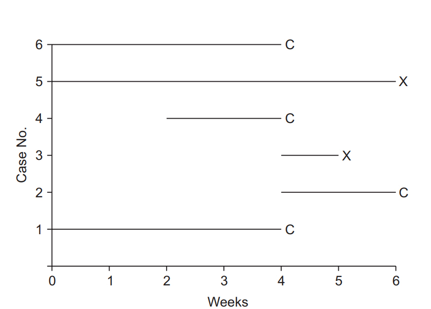
Illustration of survival analysis data from an imaginary experiment with a 6-week study period. Cases 3 and 5 experienced the event and are coded as “event cases”, denoted “X”. Their follow-up periods were 6 and 1 weeks, respectively. The others are all “censored cases,” denoted “C.” Patient 1 participated in the study from the start, but the follow-up was terminated due to unexpected death from an irrelevant cause. Patient 2 participated in the study from 4 to 6 weeks, but then refused to participate further. Case 4 was enrolled in the study in the 2nd week, lost contact in the 4th week, and was considered lost to follow-up. Case 6 was excluded in the 4th week because of uncovered random allocation.
kja-d-18-00067f1.jpg
Fig. 2.
Data arranged for Kaplan-Meier analysis. Note that for all participants the observations are rearranged to start at zero. Events are denoted “X,” and censored data are denoted “C.”
kja-d-18-00067f2.jpg
Fig. 3.
Example of a Kaplan-Meier survival curve. The axes represent time (x-axis) and survival rate (y-axis). At every time point of event occurrence, the survival curve steps down to the next lower level. Black dots represent points of censored data. At the bottom of the graph, the number of risk and censored cases are presented. It is recommended that specify these numbers with adequate time interval to clarify the clinical meanings.
kja-d-18-00067f3.jpg
Fig. 4.
Kaplan-Meier curves for groups A and B. The median survival time (postoperative nausea and vomiting-free time) for group A was 13.0 h (Q1, Q3: 8.0, 24.0 h), and for group B 6.0 h (Q1, Q3: 3.0, 17.0 h). The median survival time was significantly longer in group A than in group B (log-rank test, χ2 (1) = 6.802, P = 0.009). Black crosses indicate censored data.
kja-d-18-00067f4.jpg
Fig. 5.
Cumulative survival curves of groups A and B estimated using the Cox proportional hazards regression model. The survival curve of group B decreases considerably compared to that of group A as time passes. The hazard ratio for antiemetics was estimated as 2.0 (95% CI: 1.2–3.3, P = 0.009). Group B showed a 2-fold greater hazard of postoperative nausea and vomiting (PONV) compared to group A. Intraoperative fentanyl increased the PONV risk about 4.7-fold (95% CI: 2.8–8.1, P < 0.001) compared to non-use.
kja-d-18-00067f5.jpg
Fig. 6.
Log-log function curves for the antiemetic comparison experiment. The Y-axis represents the log-log transformed survival function estimated using the Cox proportional hazards regression model. The basic assumption of Cox proportional hazards regression modeling, a constant hazard ratio over the time (the proportional hazards assumption), can be checked using this plot for only one covariate, the antiemetic. The two curves do not cross over in the early period of observation and remain parallel after that. This plot suggests that this model does not violate the proportional hazards assumption (Created with: IBM® SPSS® Statistics ver. 23 [IBM Corp., USA]).
kja-d-18-00067f6.jpg
Table 1.
Sample of Imaginary Data from an Experiment Testing Two Antiemetics for Use in Controlling Postoperative Nausea and Vomiting
No Antiemetic Age (yr) Weight (kg) Opioid used Onset time (h) PONV Event Inclusion
1 A 48 78.5 Remifentanil 4 Not reported Censored Excluded
2 B 48 86.7 Remifentanil 17 Reported Event Included
3 A 54 88.3 Fentanyl 21 Not reported Censored Excluded
25 B 77 53 Remifentanil 24 Not reported Censored Included
104 B 58 60 Fentanyl 1 Reported Event Included

In this imaginary experiment, two antiemetics (A or B) were administered, and each patient was randomly allocated to a group receiving one of them. Intraoperative opioid used was recorded in the “opioid used” column. Postoperative nausea and vomiting (PONV) and its onset time were also recorded. For statistical tests such as Student’s t-test, patients 1 and 3 patients would normally be excluded (as indicated in the column labeled “Inclusion”). For survival analysis, all the patients would be included either as censored cases (numbers 1, 3, 25) or as ordinary event cases (numbers 2, 104).

Table 2.
Demographic Data of Patients in the Imaginary Experiment Described in Table 1
Variables Group A Group B
Number of patients 51 53
Age (yr) 56.1 (13.7) 61.2 (14.9)
Body weight (kg) 65.7 (13.8) 57.7 (11.6)
Observation time (h) 11.3 (6.7) 8.9 (7.7)
Fentanyl used 19 (37.3%) 22 (41.5%)

All data are presented as mean (SD) or number (%).

Table 3.
Estimated Hazard Ratio of Each Covariate Included in Cox Proportional Hazards Regression Modeling
Variables Hazard ratio P value
Antiemetic 1.95 (95% CI: 1.14–3.33) 0.014*
Age 0.99 (95% CI: 0.98–1.01) 0.494
Weight 0.99 (95% CI: 0.97–1.02) 0.612
Opioid used 4.87 (95% CI: 2.82–8.39) < 0.001*

“Antiemetic” and “Opioid used” showed statistically significant hazard ratios. To enhance comprehension, all hazard ratios are presented with 2 decimal points. According to this result, stepwise regression should be carried out.

References

1. Kleinbaum DG, Klein M. Survival Analysis. A Self-Learnin Text. 2nd ed. New York, Springer Science+Business Median, Inc. 2005, pp 4-5.

2. Hancock MJ, Maher CG, Costa Lda C, Williams CM. A guide to survival analysis for manual therapy clinicians and researchers. Man Ther 2014; 19: 511-6.
crossref pmid
3. Kim JM, Lee H, Ha T, Na S. Perioperative factors associated with pressure ulcer development after major surgery. Korean J Anesthesiol 2018; 71: 48-56.
crossref pmid
4. Lee JH, Kang SH, Kim Y, Kim HA, Kim BS. Effects of propofol-based total intravenous anesthesia on recurrence and overall survival in patients after modified radical mastectomy: a retrospective study. Korean J Anesthesiol 2016; 69: 126-32.
crossref pmid pmc
5. Shim JH, Jeon WJ, Cho SY, Choe GH. Comparison of the GlideScope and the McGrath method using vascular forceps and a tube exchanger in cases of simulated difficult airway intubation. Korean J Anesthesiol 2016; 69: 133-7.
crossref pmid pmc
6. Leung KM, Elashoff RM, Afifi AA. Censoring issues in survival analysis. Annu Rev Public Health 1997; 18: 83-104.
crossref pmid
7. Clark TG, Bradburn MJ, Love SB, Altman DG. Survival analysis part I: basic concepts and first analyses. Br J Cancer 2003; 89: 232-8.
crossref pmid pmc pdf
8. Selvin S. Survival analysis for epidemiologic and medical research: a practical guide. Cambridge, Cambridge university press. 2008, pp 1-26.

9. Zwiener I, Blettner M, Hommel G. Survival analysis: part 15 of a series on evaluation of scientific publications. Dtsch Arztebl Int 2011; 108: 163-9.
crossref pmid pmc
10. Goel MK, Khanna P, Kishore J. Understanding survival analysis: Kaplan-Meier estimate. Int J Ayurveda Res 2010; 1: 274-8.
crossref pmid pmc
11. Backman S, Baker A, Beattie S, Brasher P, Bryson G, Cheng D, et al. 2011 Canadian Journal of Anesthesia Guide for Authors. Can J Anesth 2011; 58: 668-96.
crossref pdf
12. Mathew A, Pandey M, Murthy NS. Survival analysis: caveats and pitfalls. Eur J Surg Oncol 1999; 25: 321-9.
crossref pmid
13. Zwiener I, Blettner M, Hommel G. Survival analysis: part 15 of a series on evaluation of scientific publications. Dtsch Arztebl Int 2011; 108: 163-9.
crossref pmid pmc
14. Bewick V, Cheek L, Ball J. Statistics review 12: survival analysis. Crit Care 2004; 8: 389-94.
crossref pmid pmc
15. Macin D, Cheung YB, Parmar MK. Survival analysis – A practical approach. 2nd ed. West Sussex, John Wiley & Sons, Ltd. 2006, pp 226-9.

16. Ishak KJ, Kreif N, Benedict A, Muszbek N. Overview of parametric survival analysis for health-economic applications. Pharmacoeconomics 2013; 31: 663-75.
crossref pmid
17. Bradburn MJ, Clark TG, Love SB, Altman DG. Survival analysis part II: multivariate data analysis--an introduction to concepts and methods. Br J Cancer 2003; 89: 431-6.
crossref pmid pmc pdf
18. George B, Seals S, Aban I. Survival analysis and regression models. J Nucl Cardiol 2014; 21: 686-94.
crossref pmid pmc
19. Ng'andu NH. An empirical comparison of statistical tests for assessing the proportional hazards assumption of Cox's model. Stat Med 1997; 16: 611-26.
crossref pmid
20. Abraira V, Muriel A, Emparanza JI, Pijoan JI, Royuela A, Plana MN, et al. Reporting quality of survival analyses in medical journals still needs improvement. A minimal requirements proposal. J Clin Epidemiol 2013; 66: 1340-6.
crossref pmid
21. Macin D, Cheung YB, Parmar MK. Survival analysis – A practical approach. 2nd ed. West Sussex, John Wiley & Sons, Ltd. 2006, pp 223-5.

22. Schmidt R, Kwiecien R, Faldum A, Berthold F, Hero B, Ligges S. Sample size calculation for the one-sample log-rank test. Stat Med 2015; 34: 1031-40.
crossref pmid
23. Schmoor C, Sauerbrei W, Schumacher M. Sample size considerations for the evaluation of prognostic factors in survival analysis. Stat Med 2000; 19: 441-52.
crossref pmid
24. Julious SA. Sample sizes for clinical trials. Boca Raton, CRC Press. 2009, pp 63-9.


ABOUT
ARTICLE CATEGORY

Browse all articles >

BROWSE ARTICLES
AUTHOR INFORMATION
Editorial Office
101-3503, Lotte Castle President, 109 Mapo-daero, Mapo-gu, Seoul 04146, Korea
(서울특별시 마포구 마포대로 109 롯데캐슬 프레지던트 101동 3503호)
Tel: +82-2-792-5128    Fax: +82-2-792-4089    E-mail: journal@anesthesia.or.kr                
Business Name: Korean Society of Anesthesiologists (대한마취통증의학회)
Business Registration: 106-82-07194
Representative: Jun Heum Yon (연준흠)

Copyright © 2024 by Korean Society of Anesthesiologists.

Developed in M2PI

Close layer
prev next