


Introduction
Most parametric statistical analysis methods require normality assumptions. When violated, statistical results from non-normally distributed data could be a cause of serious error. These are apparent obstacles for confident scientific results. Even though the central limit theory could cover normality when the size of the sample is sufficient, many clinical and experimental data fail to satisfy normality assumptions despite a relatively large sample size. Fortunately, a simple statistical technique, variable transformation, provides a method to convert data distribution from non-normal to normal. Furthermore, the variable transformation could form a linear relationship between variables from a non-linear relationship and could stabilize estimated variance in linear modeling.
Although variable transformation provides an appropriate method of parametric statistical analysis, interpretation of inferred results is quite a different problem. Variable transformation changes the distribution of data as well as its original unit of measure [1]. To interpret such results or to compare the results with others, back-transformation is essential. Statistical analysis always assumes that there is a permissive error within the alpha limit because it is based on the probability. Back-transformation of error term included in statistical analysis requires complicated processes when sophisticated transformation methods are applied.
This article covers general concepts of variable transformation, logarithmic transformation and back transformation that could be useful in medical statistics, and concepts of power transformation, especially about Box-Cox transformation. Finally, descriptions of general precautions when considering variable transformation are provided.
Distribution of each variable and relationship between variables
Before commencing statistical analysis, checking data distribution, the relationship between variables, missing data, and outlier controlling are appropriate method of statistical analysis and inference, which allow us to overcome issues that may occur during analysis. Data distribution and relationships between variables determine unsuitable variables of skewed distribution and reveal the possibility of planned linear regression.
The shape of data distribution is often couched in terms of representative values, including mean, median, and values of dispersion such as standard deviation (SD), quartiles, range, maximum, and minimum. In addition, skewness and kurtosis reveals the more detailed shape of data distribution [2] and most statistical software provides extensive information about these factors. If one variable violates the normality assumption, distribution plot or skewness/kurtosis provide a clue regarding data distribution (Table 1).
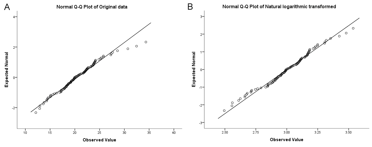
A quantile-quantile plot (Q-Q plot) with a normality test could imply the skewness of data distribution [3]. Normally distributed data appears as a rough straight line while skewed data presents a curved line on a Q-Q plot (Fig. 1).
In a clinical situation, various data follow positively or negatively skewed distributions. For example, in terms of mean arterial pressure, most people have normal blood pressure and some patients with hypertension would present higher mean arterial pressure with a small portion of aggregate data. Randomly sampled mean arterial pressure data from the general population will have a positively skewed distribution. Plasma hemoglobin concentration from the general population will have a negatively skewed distribution if the incidence of anemia is higher than polycythemia.
According to the characteristics of data distribution, various transformation methods can be used to achieve satisfaction for the normality test (Table 1). These kinds of transformations could make the data symmetrically distributed and the absolute value of the skewness close to zero [1]. These transformation methods could be applied to ensure the linear relationship between variables. It is well known that many statistical modeling methods are based on the linear relationship between treatment and response variables, and forming an apparent linear relationship through variable transformation enhances statistical model estimation. A typical example is logit transformation, which is used for binomial logistic regression. The logit transformation converts the probability of an event to log odds, allowing regression analysis between the dichotomous outcome variable and the independent variable, which plays the role of the linear predictor. The odds ratio can be used to interpret logit transformed regression. However, if a transformation is conducted with a variable using complex methods or if treatment and response variables are simultaneously transformed, interpretation of estimated results may be challenging. Therefore, transformation should remain as simple as possible to ensure a comprehensive interpretation of statistically inferred results.
Non-linear transformations
Adding, subtracting, multiplying, or dividing with a constant is commonly considered as the linear transformation, because these transformations rarely affect the distribution of data, they only shift the geometric mean and SD to some extent by their nature. In contrast, other transformations, including logarithmic transformation are referred to as non-linear transformation. They stabilize dispersion, create a linear relationship between variables, and enable parametric statistical estimation with the normality assumption assured.
Although these transformation methods provide a satisfying statistical result, the transformation itself forms an obstacle in terms of interpreting and reporting the statistical results. The transformed variable itself is sometimes meaningful without back-transformation. For example, a certain cancer incidence is proportional to the square of the smoking period. This result is based on the linear regression analysis with observed cancer incidence and squared period of smoking, and its interpretation has meaning without back-transformation. We can present the collected data with median and 1st and 3rd quartiles of the smoking period when the original data have violated the normality assumption. If we compare the smoking periods between two groups and they require square transformation to keep the normality assumption, it is hard to interpret the clinical meaning of the mean difference of squared data. The difference between each squared value is not the same as the squared difference between the two original scaled values. In this situation, non-parametric analysis makes it easier to interpret the results.
A non-linear transformation may sometimes be required to obey the assumptions for a specific statistical analysis such as multiple linear regression. If we use undiscerning transformation methods for numerous variables, it is hard to interpret estimated results. For complex statistical analysis, it is therefore better to use an interpretable transformation method. In addition, using a more liberal statistical method such as generalized linear or non-linear models may be more appropriate.
Logarithmic transformation
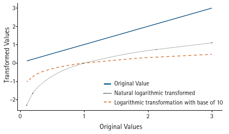
Applying a logarithmic transformation, each value is changed by the characteristics of the logarithm. Considering its features, the differences between transformed values become smaller than the original scale (Fig. 2). The logarithmic transformation compresses the differences between the upper and lower part of the original scale of data. For example, for data with 100 cases, its skewness of 0.56 changes to -0.14 after natural logarithmic transformation. The results of the normality test using the Shapiro-Wilk test also changes its statistics from 0.974 (P = 0.047) to 0.988 (P = 0.477). The Q-Q plot also is stabilized after logarithmic transformation (Fig. 1). As shown here, a logarithmic transformation has a normalizing effect on the positively skewed distribution. This transformed distribution is referred to as ‘log-normal distribution.’ An interesting finding from the logarithmic transformation is that its effects cover normalizing the density of data and decreasing the SD, the latter provides greater opportunity to satisfy the equal variance test, which is frequently used for various parametric statistical inferences. From Fig. 1, the mean and SD of the original data are 20.52 and 4.117 become 3.0 and 0.201 after logarithmic transformation. The coefficients of variances are 20.1% and 7.0% for original and logarithmically transformed data, respectively. The coefficient of variance is a representative value for a standardized measure of the dispersion of data distribution. A large value implies that one value from the data has a high risk of being far from the mean. With decreased SDs, the results of the equal variance test could be satisfied, and several comparison methods including Student’s t-test could be possible after logarithmic transformation of a variable1).
Although we can generate the data for intended statistical analysis, the interpretation of statistically inferred data is another obstacle. If we present the inferred data with a transformed scale, it is not easy to understand the results themselves. We therefore need back-transformation, which is the exponential transformation [4], for the statistical results. If we use natural logarithmic transformation, then back-transformation requires natural exponential function. The calculation is simple, but interpretation is difficult. The mean value of logarithmic transformation should be converted to an exponential scale. Means of original and transformed data are 20.53 and e3.00 = 20.09, respectively (Fig. 1). The mean value of 20.09, which is known as the geometric mean, is the back-transformed mean value from transformed data. The geometric mean is less affected by the very large values of original data than the corresponding arithmetic mean, which comes from a skewed distribution. SD should also be considered for back-transformation from estimated values. However, for the moment of back-transformation, the meaning of ‘standard’ deviation loses its additive meaning because such data are not normally distributed [5]. Its interpretation does not make sense after back-transformation. Hence, the CI is usually reported for this situation [4,6]. A back-transformed CI allows better understanding on the original scaled data. For example, the mean and SD are 3.00 and 0.201 for natural logarithmic transformed data with a sample size of 100 and its 95% CI is from 2.96 to 3.03. When back-transformation is performed with an exponential function, it changes into from 19.31 to 20.89. Considering the geometric mean is 20.09, a back-transformed 95% CI does not have symmetric placement from the geometric mean value. We sometimes use a variable with the transformed form by default. Back-transformation is essential for statistical analysis and should be returned to its original scale when reporting the results. The one example is the antibody titer. If one patient with myasthenia gravis tested positive for anticholinesterase with an antibody titer 1:32, it means that the number of dilutions should be repeated five times until the last seropositive results (25 = 32). Antibody titer itself has a characteristic of the powered value of dilution numbers, which is always is reported as 1:2dilution numbers. Hence, the geometric mean should be presented as 2mean dilution number, not the mean of titers.
Furthermore, mean difference obtained from the t-test does not imply a simple difference between estimated means when a logarithmic transformation is used. Back-transformation from logarithmic transformation leads to arithmetic difference of transformed variables to ratio. The mean difference from two natural logarithmic transformed samples is X1-X2, and back-transformation results in e X 1 - X 2 = e X 1 / e X 2
Pearson’s correlation analysis and linear regression analysis also require data normality. When the logarithmic transformation is applied to the data for the former, the result can be described as estimated. The correlation coefficient is a statistic that has the characteristics of effect size, and we do not need to conduct further back-transformation. Only one thing should be done reporting results with the information about transformation. If logarithmic transformation is applied for linear regression, it produces more complex considerations in terms of results interpretation. Linear regression requires several assumptions, including the linear relationship between independent and dependent variables. To fulfill this assumption, variable transformation may be necessary. If the dependent variable requires logarithmic transformation, the meaning of the regression coefficient changes from unit change to a ratio. Basically, the definition of the regression coefficient is that ‘a one-unit change in the independent variable produces an increase (decrease) in the dependent variable by the amount of regression coefficient.’ Arithmetic increment (decrement) of the transformed dependent variable will be changed into a ratio with back-transformation of an exponential function. For example, the estimated regression coefficient is 0.1, e0.1 = 1.105, means ‘for a one-unit increase in the independent variable, dependent variable increases by 10.5%.’ Similar to the explanation of the mean difference, it should be noted that the interpreted value is not 110.5%. If the dependent variable is a common logarithmic transformed variable, a one-unit change in the independent variable is the same as a tenfold increment in the original matric variable. That is, a tenfold increment in independent variable produces dependent variable changes by the estimated regression coefficient. Description with a 1% increment of the independent variable is also possible. For the convenience, common logarithmic transformation is better for independent variable transformation. If natural logarithmic transformation is applied, interpretation is not easy with e as the base of the natural logarithm; the approximated value is 2.71828. If both dependent and independent variables are transformed with logarithmic transformation, we can interpret the result as a percentile increment of the independent variable produces a percentile change in the dependent variable following the rule explained above. These interpretation rules can be applied to the other kind of general linear modeling method including ANCOVA and MANOVA.
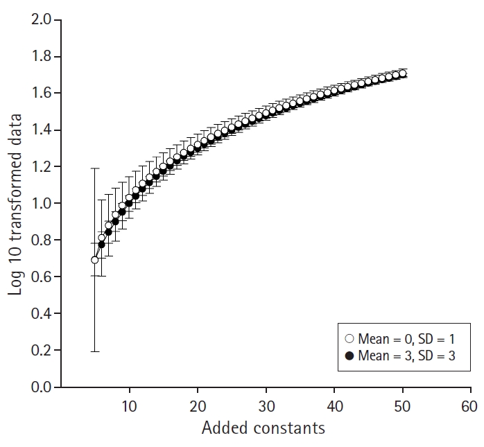
Several problems are reported regarding logarithmic transformation [7]. Such transformation is impossible when the values have negative or zero in its original metric. To overcome this problem, adding a positive constant to the original data is a common practice. However, the shape of the logarithmic graph subtly changes in the early stage from zero and then enters the fluent curve section in the later stage (Fig. 2). That is, the dispersion of logarithmically transformed data could be varied according to the added value from original scaled data. For example, assume two normally distributed data sets with mean = 0, SD = 1, n =100 and mean =1, SD = 3, n =100 using a random number creation function. Then, we add the integers that make all data have positive values. Logarithmic transformation with a base of 10 is applied to all datasets. Then, plotting their mean and SD in one graph, we can see the mean differences and SDs become smaller according to an increment of an added constant (Fig. 3). As a result, estimated t-statistics and P values are also changed, which increases the statistical errors. These kinds of errors could only occur when the mean difference and SD are relatively small, but estimated t-statistic could increase as the added value increases even if mean difference and SD are large. These kinds of errors originate from the nature of logarithmic transformation; it increases the difference when the values are small and reduces the difference when the values are large. From the null hypothesis significance testing viewpoint, the significance of the t-test may not change except when t-statistics are very near to the significance level. However, it should be noted that estimated statistics and performed power also change because logarithmic transformation stabilizes SD values.
Power transformation and Box-Cox transformation
Power transformation is a transformation method that uses a power function. If we use a number greater than 1 as an index of a power function, it could transform left-skewed data into near-normally distributed data. A specialized form of power transformation is the Box-Cox transformation [8], which is frequently applied to stabilize the variance of errors estimated during linear regression or correlation analysis. There are several extended forms of Box-Cox transformation [9], the traditional method is as shown in (Equation 1) below.
According to the value of λ, this performs various types of non-linear transformation. For example, λ = -1 produces a reciprocal transformation, λ = 2 a square transformation, and λ = 0.5 a square root transformation. Because it contains a constant, a somewhat linear transformation is also applied as we already know the linear transformation hardly effects the estimated statistics. However, we should be cautious as such transformation could affect the statistical results, as described in the previous section. If λ = 0, the Box-Cox transformation is same as logarithmic transformation. Then, how can we determine the value of λ and how the Box-Cox transformation stabilizes the variance? We consider this using linear regression. Linear regression requires several assumptions including homoscedasticity, which means all observed values are equally scattered from the estimated regression line. Several residual diagnostics provide about homoscedasticity. When the homoscedasticity is violated, the Box-Cox transformation could stabilize the variance of residuals. Using yλ instead of y in the linear regression model, for example, yλ = αx + β + ε (α: regression coefficient, β: constant, ε: error), several statistical software programs2) find best estimated values of λ and its 95% CI based on the maximal likelihood method. Using this result, we can estimate the linear regression model with homoscedasticity. Although the Box-Cox transformation is an excellent tool to obtain the best results of linear regression, it also has a serious problem of result interpretation. Back-transformation for this is not as simple as other non-linear transformations because it includes the error term, which is essential for the linear regression. There are several proposed back-transformation methods from the Box-Cox transformation [10,11], which require complex statistical process. If we try to interpret as the transformed variable itself, we should also consider the transformed unit, which could lose its real meaning after transformation. Only when the other measures for stabilizing variance (homoscedasticity) have failed, should the Box-Cox transformation be considered.
Conclusion
Parametric statistical analysis is frequently used in medical research. Unfortunately, many physicians have not recognized that these analytic methods require the normality of data distribution and other assumptions. There are many other analytic methods with more generous assumptions such as generalized linear or non-linear models. Nevertheless, we need simplified and intuitive analysis, including t-test and analysis of variances (ANOVA). Variable transformation is a powerful tool to make data normally distributed or to form a linear relationship of data. However, almost all of the transformed data should be back-transformed for the interpretation of the results. The transformation could be easy, it is possible to calculate the transformation in commonly used spreadsheet programs. However, back-transformation is not an easy process if complex or a combination of several transformations are used. Result interpretation also depends on the role of the transformed variable. It is relatively simple for a transformed independent variable to be compared to the transformed dependent variable. When the dependent variable is transformed, back-transformation should rely on the transformed error term.
Variable transformation provides an attractive and convenient method of enabling parametric statistical analysis, and data preparation should be considered a priori. Information about data distribution, such as skewness, range, mean, SD, median, and quartiles, and the relationship between variables (scatter plot) can be used to derive the best method. Outlier controlling, missing data evaluation, and adequacy of sample size should be prioritized before variable transformation. If possible, using statistical analysis with generous assumptions is an option and non-parametric statistical analysis also guarantees a scientific result.