


Introduction
A t test is a type of statistical test that is used to compare the means of two groups. It is one of the most widely used statistical hypothesis tests in pain studies [1]. There are two types of statistical inference: parametric and nonparametric methods. Parametric methods refer to a statistical technique in which one defines the probability distribution of probability variables and makes inferences about the parameters of the distribution. In cases in which the probability distribution cannot be defined, nonparametric methods are employed. T tests are a type of parametric method; they can be used when the samples satisfy the conditions of normality, equal variance, and independence.
T tests can be divided into two types. There is the independent t test, which can be used when the two groups under comparison are independent of each other, and the paired t test, which can be used when the two groups under comparison are dependent on each other. T tests are usually used in cases where the experimental subjects are divided into two independent groups, with one group treated with A and the other group treated with B. Researchers can acquire two types of results for each group (i.e., prior to treatment and after the treatment): preA and postA, and preB and postB. An independent t test can be used for an intergroup comparison of postA and postB or for an intergroup comparison of changes in preA to postA (postA-preA) and changes in preB to postB (postB-preB) (Table 1).
On the other hand, paired t tests are used in different experimental environments. For example, the experimental subjects are not divided into two groups, and all of them are treated initially with A. The amount of change (postA-preA) is then measured for all subjects. After all of the effects of A disappear, the subjects are treated with B, and the amount of change (postB-preB) is measured for all of the subjects. A paired t test is used in such crossover test designs to compare the amount of change of A to that of B for the same subjects (Table 2).
Statistic and Probability
Statistics is basically about probabilities. A statistical conclusion of a large or small difference between two groups is not based on an absolute standard but is rather an evaluation of the probability of an event. For example, a clinical test is performed to determine whether or not a patient has a certain disease. If the test results are either higher or lower than the standard, clinicians will determine that the patient has the disease despite the fact that the patient may or may not actually have the disease. This conclusion is based on the statistical concept which holds that it is more statistically valid to conclude that the patient has the disease than to declare that the patient is a rare case among people without the disease because such test results are statistically rare in normal people.
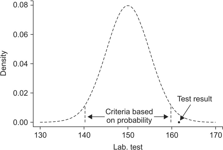
The test results and the probability distribution of the results must be known in order for the results to be determined as statistically rare. The criteria for clinical indicators have been established based on data collected from an entire population or at least from a large number of people. Here, we examine a case in which a clinical indicator exhibits a normal distribution with a mean of µ and a variance of σ2. If a patient's test result is χ, is this statistically rare against the criteria (e.g., 5 or 1%)? Probability is represented as the surface area in a probability distribution, and the z score that represents either 5 or 1%, near the margins of the distribution, becomes the reference value. The test result χ can be determined to be statistically rare compared to the reference probability if it lies in a more marginal area than the z score, that is, if the value of χ is located in the marginal ends of the distribution (Fig. 1).
This is done to compare one individual's clinical indicator value. This however raises the question of how we would compare the mean of a sample group (consisting of more than one individual) against the population mean. Again, it is meaningless to compare each individual separately; we must compare the means of the two groups. Thus, do we make a statistical inference using only the distribution of the clinical indicators of the entire population and the mean of the sample? No. In order to infer a statistical possibility, we must know the indicator of interest and its probability distribution. In other words, we must know the mean of the sample and the distribution of the mean. We can then determine how far the sample mean varies from the population mean by knowing the sampling distribution of the means.
Sampling Distribution (Sample Mean Distribution)
The sample mean we can get from a study is one of means of all possible samples which could be drawn from a population. This sample mean from a study was already acquired from a real experiment, however, how could we know the distribution of the means of all possible samples including studied sample? Do we need to experiment it over and over again? The simulation in which samples are drawn repeatedly from a population is shown in Fig. 2. If samples are drawn with sample size n from population of normal distribution (µ, σ2), the sampling distribution shows normal distribution with mean of µ and variance of σ2/n. The number of samples affects the shape of the sampling distribution. That is, the shape of the distribution curve becomes a narrower bell curve with a smaller variance as the number of samples increases, because the variance of sampling distribution is σ2/n. The formation of a sampling distribution is well explained in Lee et al. [2] in a form of a figure.
T Distribution
Now that the sampling distribution of the means is known, we can locate the position of the mean of a specific sample against the distribution data. However, one problem remains. As we noted earlier, the sampling distribution exhibits a normal distribution with a variance of σ2/n, but in reality we do not know σ2, the variance of the population. Therefore, we use the sample variance instead of the population variance to determine the sampling distribution of the mean. The sample variance is defined as follows:
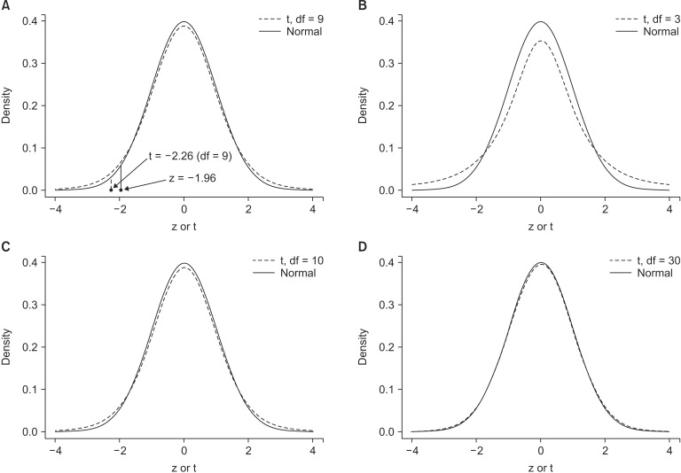
In such cases in which the sample variance is used, the sampling distribution follows a t distribution that depends on the 0degree of freedom of each sample rather than a normal distribution (Fig. 3).
Independent T test
A t test is also known as Student's t test. It is a statistical analysis technique that was developed by William Sealy Gosset in 1908 as a means to control the quality of dark beers. A t test used to test whether there is a difference between two independent sample means is not different from a t test used when there is only one sample (as mentioned earlier). However, if there is no difference in the two sample means, the difference will be close to zero. Therefore, in such cases, an additional statistical test should be performed to verify whether the difference could be said to be equal to zero.
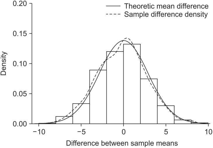
Let's extract two independent samples from a population that displays a normal distribution and compute the difference between the means of the two samples. The difference between the sample means will not always be zero, even if the samples are extracted from the same population, because the sampling process is randomized, which results in a sample with a variety of combinations of subjects. We extracted two samples with a size of 6 from a population N (150, 52) and found the difference in the means. If this process is repeated 1,000 times, the sampling distribution exhibits the shape illustrated in Fig. 4. When the distribution is displayed in terms of a histogram and a density line, it is almost identical to the theoretical sampling distribution: N(0, 2 × 52/6) (Fig. 4).
However, it is difficult to define the distribution of the difference in the two sample means because the variance of the population is unknown. If we use the variance of the sample instead, the distribution of the difference of the samples means would follow a t distribution. It should be noted, however, that the two samples display a normal distribution and have an equal variance because they were independently extracted from an identical population that has a normal distribution.
Under the assumption that the two samples display a normal distribution and have an equal variance, the t statistic is as follows:
The population variance was unknown and so a pooled variance of the two samples was used:
However, if the population variance is not equal, the t statistic of the t test would be
and the degree of freedom is calculated based on the Welch Satterthwaite equation.
It is apparent that if n1 and n2 are sufficiently large, the t statistic resembles a normal distribution (Fig. 3).
A statistical test is performed to verify the position of the difference in the sample means in the sampling distribution of the mean (Fig. 4). It is statistically very rare for the difference in two sample means to lie on the margins of the distribution. Therefore, if the difference does lie on the margins, it is statistically significant to conclude that the samples were extracted from two different populations, even if they were actually extracted from the same population.
Paired T test
Paired t tests are can be categorized as a type of t test for a single sample because they test the difference between two paired results. If there is no difference between the two treatments, the difference in the results would be close to zero; hence, the difference in the sample means used for a paired t test would be 0.
Let's go back to the sampling distribution that was used in the independent t test discussed earlier. The variance of the difference between two independent sample means was represented as the sum of each variance. If the samples were not independent, the variance of the difference of two variables A and B, Var (A-B), can be shown as follows,
where σ12 is the variance of variable A, σ22 is the variance of variable B, and ρ is the correlation coefficient for the two variables. In an independent t test, the correlation coefficient is 0 because the two groups are independent. Thus, it is logical to show the variance of the difference between the two variables simply as the sum of the two variances. However, for paired variables, the correlation coefficient may not equal 0. Thus, the t statistic for two dependent samples must be different, meaning the following t statistic,
must be changed. First, the number of samples are paired; thus, n1 = n2 = n, and their variance can be represented as s12 + s22 - 2ρs1s2 considering the correlation coefficient. Therefore, the t statistic for a paired t test is as follows:
In this equation, the t statistic is increased if the correlation coefficient is greater than 0 because the denominator becomes smaller, which increases the statistical power of the paired t test compared to that of an independent t test. On the other hand, if the correlation coefficient is less than 0, the statistical power is decreased and becomes lower than that of an independent t test. It is important to note that if one misunderstands this characteristic and uses an independent t test when the correlation coefficient is less than 0, the generated results would be incorrect, as the process ignores the paired experimental design.
Assumptions
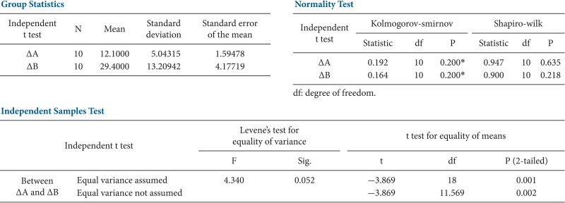
As previously explained, if samples are extracted from a population that displays a normal distribution but the population variance is unknown, we can use the sample variance to examine the sampling distribution of the mean, which will resemble a t distribution. Therefore, in order to reach a statistical conclusion about a sample mean with a t distribution, certain conditions must be satisfied: the two samples for comparison must be independently sampled from the same population, satisfying the conditions of normality, equal variance, and independence.
Shapiro's test or the Kolmogorov-Smirnov test can be performed to verify the assumption of normality. If the condition of normality is not met, the Wilcoxon rank sum test (Mann-Whitney U test) is used for independent samples, and the Wilcoxon sign rank test is used for paired samples for an additional nonparametric test.
The condition of equal variance is verified using Levene's test or Bartlett's test. If the condition of equal variance is not met, nonparametric test can be performed or the following statistic which follows a t distribution can is used.
Conclusion
Owing to user-friendly statistics software programs, the rich pool of statistics information on the Internet, and expert advice from statistics professionals at every hospital, using and processing statistics data is no longer an intractable task. However, it remains the researchers' responsibility to design experiments to fulfill all of the conditions of their statistic methods of choice and to ensure that their statistical assumptions are appropriate. In particular, parametric statistical methods confer reasonable statistical conclusions only when the statistical assumptions are fully met. Some researchers often regard these statistical assumptions inconvenient and neglect them. Even some statisticians argue on the basic assumptions, based on the central limit theory, that sampling distributions display a normal distribution regardless of the fact that the population distribution may or may not follow a normal distribution, and that t tests have sufficient statistical power even if they do not satisfy the condition of normality [5]. Moreover, they contend that the condition of equal variance is not so strict because even if there is a ninefold difference in the variance, the α level merely changes from 0.5 to 0.6 [6]. However, the arguments regarding the conditions of normality and the limit to which the condition of equal variance may be violated are still bones of contention. Therefore, researchers who unquestioningly accept these arguments and neglect the basic assumptions of a t test when submitting papers will face critical comments from editors. Moreover, it will be difficult to persuade the editors to neglect the basic assumptions regardless of how solid the evidence in the paper is. Hence, researchers should sufficiently test basic statistical assumptions and employ methods that are widely accepted so as to draw valid statistical conclusions.