


Multiple Comparison Test and Its Imitations
We are not always interested in comparison of two groups per experiment. Sometimes (in practice, very often), we may have to determine whether differences exist among the means of three or more groups. The most common analytical method used for such determinations is analysis of variance (ANOVA). 1) When the null hypothesis (H0) is rejected after ANOVA, that is, in the case of three groups, H0: μA = μB = μC, we do not know how one group differs from a certain group. The result of ANOVA does not provide detailed information regarding the differences among various combinations of groups. Therefore, researchers usually perform additional analysis to clarify the differences between particular pairs of experimental groups. If the null hypothesis (H0) is rejected in the ANOVA for the three groups, the following cases are considered:
In which of these cases is the null hypothesis rejected? The only way to answer this question is to apply the ‘multiple comparison test’ (MCT), which is sometimes also called a ‘post-hoc test.’
There are several methods for performing MCT, such as the Tukey method, Newman-Keuls method, Bonferroni method, Dunnett method, Scheffé’s test, and so on. In this paper, we discuss the best multiple comparison method for analyzing given data, clarify how to distinguish between these methods, and describe the method for adjusting the P value to prevent α inflation in general multiple comparison situations. Further, we describe the increase in type I error (α inflation), which should always be considered in multiple comparisons, and the method for controlling type I error that applied in each corresponding multiple comparison method.
Meaning of P value and ɑ Inflation
In a statistical hypothesis test, the significance probability, asymptotic significance, or P value (probability value) denotes the probability that an extreme result will actually be observed if H0 is true. The significance of an experiment is a random variable that is defined in the sample space of the experiment and has a value between 0 and 1.
Type I error occurs when H0 is statistically rejected even though it is actually true, whereas type II error refers to a false negative, H0 is statistically accepted but H0 is false (Table 1). In the situation of comparing the three groups, they may form the following three pairs: group 1 versus group 2, group 2 versus group 3, and group 1 versus group 3. A pair for this comparison is called ‘family.’ The type I error that occurs when each family is compared is called the ‘family-wise error’ (FWE). In other words, the method developed to appropriately adjust the FWE is a multiple comparison method. The α inflation can occur when the same (without adjustment) significant level is applied to the statistical analysis to one and other families simultaneously [2]. For example, if one performs a Student’s t-test between two given groups A and B under 5% α error and significantly indifferent statistical result, the probability of trueness of H0 (the hypothesis that groups A and B are same) is 95%. At this point, let us consider another group called group C, which we want to compare it and groups A and B. If one performs another Student’s t-test between the groups A and B and its result is also nonsignificant, the real probability of a nonsignificant result between A and B, and B and C is 0.95 × 0.95 = 0.9025, 90.25% and, consequently, the testing α error is 1 − 0.9025 = 0.0975, not 0.05. At the same time, if the statistical analysis between groups A and C also has a nonsignificant result, the probability of nonsignificance of all the three pairs (families) is 0.95 × 0.95 × 0.95 = 0.857 and the actual testing α error is 1 − 0.857 = 0.143, which is more than 14%.
The inflation of probability of type I error increases with the increase in the number of comparisons (Fig. 1, equation 1). Table 2 shows the increases in the probability of rejecting H0 according to the number of comparisons.
Unfortunately, the result of controlling the significance level for MCT will probably increase the number of false negative cases which are not detected as being statistically significant, but they are really different (Table 1). False negatives (type II errors) can lead to an increase in cost. Therefore, if this is the case, we may not even want to attempt to control the significance level for MCT. Clearly, such deliberate avoidance increases the possibility of occurrence of false positive findings.
Classification (or Type) of Multiple Comparison: Single-step versus Stepwise Procedures
As mentioned earlier, repeated testing with given groups results in the serious problem known as α inflation. Therefore, numerous MCT methods have been developed in statistics over the years.2) Most of the researchers in the field are interested in understanding the differences between relevant groups. These groups could be all pairs in the experiments, or one control and other groups, or more than two groups (one subgroup) and another experiment groups (another subgroup). Irrespective of the type of pairs to be compared, all post hoc subgroup comparing methods should be applied under the significance of complete ANOVA result.3)
Usually, MCTs are categorized into two classes, single-step and stepwise procedures. Stepwise procedures are further divided into step-up and step-down methods. This classification depends on the method used to handle type I error. As indicated by its name, single-step procedure assumes one hypothetical type I error rate. Under this assumption, almost all pairwise comparisons (multiple hypotheses) are performed (tested using one critical value). In other words, every comparison is independent. A typical example is Fisher’s least significant difference (LSD) test. Other examples are Bonferroni, Sidak, Scheffé, Tukey, Tukey-Kramer, Hochberg’s GF2, Gabriel, and Dunnett tests.
The stepwise procedure handles type I error according to previously selected comparison results, that is, it processes pairwise comparisons in a predetermined order, and each comparison is performed only when the previous comparison result is statistically significant. In general, this method improves the statistical power of the process while preserving the type I error rate throughout. Among the comparison test statistics, the most significant test (for step-down procedures) or least significant test (for step-up procedures) is identified, and comparisons are successively performed when the previous test result is significant. If one comparison test during the process fails to reject a null hypothesis, all the remaining tests are rejected. This method does not determine the same level of significance as single-step methods; rather, it classifies all relevant groups into the statistically similar subgroups. The stepwise methods include Ryan-Einot-Gabriel-Welsch Q (REGWQ), Ryan-Einot-Gabriel-Welsch F (REGWF), Student-Newman-Keuls (SNK), and Duncan tests. These methods have different uses, for example, the SNK test is started to compare the two groups with the largest differences; the other two groups with the second largest differences are compared only if there is a significant difference in prior comparison. Therefore, this method is called as step-down methods because the extents of the differences are reduced as comparisons proceed. It is noted that the critical value for comparison varies for each pair. That is, it depends on the range of mean differences between groups. The smaller the range of comparison, the smaller the critical value for the range; hence, although the power increases, the probability of type I error increases.
All the aforementioned methods can be used only in the situation of equal variance assumption. If equal variance assumption is violent during the ANOVA process, pairwise comparisons should be based on the statistics of Tamhane’s T2, Dunnett’s T3, Games-Howell, and Dunnett’s C tests.
Tukey method
This test uses pairwise post-hoc testing to determine whether there is a difference between the mean of all possible pairs using a studentized range distribution. This method tests every possible pair of all groups. Initially, the Tukey test was called the ‘Honestly significant difference’ test, or simply the ‘T test,’4) because this method was based on the t-distribution. It is noted that the Tukey test is based on the same sample counts between groups (balanced data) as ANOVA. Subsequently, Kramer modified this method to apply it on unbalanced data, and it became known as the Tukey-Kramer test. This method uses the harmonic mean of the cell size of the two comparisons. The statistical assumptions of ANOVA should be applied to the Tukey method, as well.5)
Fig. 2 depicts the example results of one-way ANOVA and Tukey test for multiple comparisons. According to this figure, the Tukey test is performed with one critical level, as described earlier, and the results of all pairwise comparisons are presented in one table under the section ‘post-hoc test.’ The results conclude that groups A and B are different, whereas groups A and C are not different and groups B and C are also not different. These odd results are continued in the last table named ‘Homogeneous subsets.’ Groups A and C are similar and groups B and C are also similar; however, groups A and B are different. An inference of this type is different with the syllogistic reasoning. In mathematics, if A = B and B = C, then A = C. However, in statistics, when A = B and B = C, A is not the same as C because all these results are probable outcomes based on statistics. Such contradictory results can originate from inadequate statistical power, that is, a small sample size. The Tukey test is a generous method to detect the difference during pairwise comparison (less conservative); to avoid this illogical result, an adequate sample size should be guaranteed, which gives rise to smaller standard errors and increases the probability of rejecting the null hypothesis.
Bonferroni method: ɑ splitting (Dunn’s method)
The Bonferroni method can be used to compare different groups at the baseline, study the relationship between variables, or examine one or more endpoints in clinical trials. It is applied as a post-hoc test in many statistical procedures such as ANOVA and its variants, including analysis of covariance (ANCOVA) and multivariate ANOVA (MANOVA); multiple t-tests; and Pearson’s correlation analysis. It is also used in several nonparametric tests, including the Mann-Whitney U test, Wilcoxon signed rank test, and Kruskal-Wallis test by ranks [4], and as a test for categorical data, such as Chi-squared test. When used as a post hoc test after ANOVA, the Bonferroni method uses thresholds based on the t-distribution; the Bonferroni method is more rigorous than the Tukey test, which tolerates type I errors, and more generous than the very conservative Scheffé’s method.
However, it has disadvantages, as well, since it is unnecessarily conservative (with weak statistical power). The adjusted α is often smaller than required, particularly if there are many tests and/or the test statistics are positively correlated. Therefore, this method often fails to detect real differences. If the proposed study requires that type II error should be avoided and possible effects should not be missed, we should not use Bonferroni correction. Rather, we should use a more liberal method like Fisher’s LSD, which does not control the family-wise error rate (FWER).6) Another alternative to the Bonferroni correction to yield overly conservative results is to use the stepwise (sequential) method, for which the Bonferroni-Holm and Hochberg methods are suitable, which are less conservative than the Bonferroni test [5].
Dunnett method
This is a particularly useful method to analyze studies having control groups, based on modified t-test statistics (Dunnett’s t-distribution). It is a powerful statistic and, therefore, can discover relatively small but significant differences among groups or combinations of groups. The Dunnett test is used by researchers interested in testing two or more experimental groups against a single control group. However, the Dunnett test has the disadvantage that it does not compare the groups other than the control group among themselves at all.
As an example, suppose there are three experimental groups A, B, and C, in which an experimental drug is used, and a control group in a study. In the Dunnett test, a comparison of control group with A, B, C, or their combinations is performed; however, no comparison is made between the experimental groups A, B, and C. Therefore, the power of the test is higher because the number of tests is reduced compared to the ‘all pairwise comparison.’
On the other hand, the Dunnett method is capable of ‘twotailed’ or ‘one-tailed’ testing, which makes it different from other pairwise comparison methods. For example, if the effect of a new drug is not known at all, the two-tailed test should be used to confirm whether the effect of the new drug is better or worse than that of a conventional control. Subsequently, a one-sided test is required to compare the new drug and control. Since the two-sided or single-sided test can be performed according to the situation, the Dunnett method can be used without any restrictions.
Scheffé’s method: exploratory post-hoc method
Scheffé’s method is not a simple pairwise comparison test. Based on F-distribution, it is a method for performing simultaneous, joint pairwise comparisons for all possible pairwise combinations of each group mean [6]. It controls FWER after considering every possible pairwise combination, whereas the Tukey test controls the FWER when only all pairwise comparisons are made.7) This is why the Scheffé’s method is very conservative than other methods and has small power to detect the differences. Since Scheffé’s method generates hypotheses based on all possible comparisons to confirm significance, this method is preferred when theoretical background for differences between groups is unavailable or previous studies have not been completely implemented (exploratory data analysis). The hypotheses generated in this manner should be tested by subsequent studies that are specifically designed to test new hypotheses. This is important in exploratory data analysis or the theoretic testing process (e.g., if a type I error is likely to occur in this type of study and the differences should be identified in subsequent studies). Follow-up studies testing specific subgroup contrasts discovered through the application of Scheffé’s method should use. Bonferroni methods that are appropriate for theoretical test studies. It is further noted that Bonferroni methods are less sensitive to type I errors than Scheffé’s method. Finally, Scheffé’s method enables simple or complex averaging comparisons in both balanced and unbalanced data.
Violation of the assumption of equivalence of variance
One-way ANOVA is performed only in cases where the assumption of equivalence of variance holds. However, it is a robust statistic that can be used even when there is a deviation from the equivalence assumption. In such cases, the Games-Howell, Tamhane’s T2, Dunnett’s T3, and Dunnett’s C tests can be applied.
The Games-Howell method is an improved version of the Tukey-Kramer method and is applicable in cases where the equivalence of variance assumption is violated. It is a t-test using Welch’s degree of freedom. This method uses a strategy for controlling the type I error for the entire comparison and is known to maintain the preset significance level even when the size of the sample is different. However, the smaller the number of samples in each group, the it is more tolerant the type I error control. Thus, this method can be applied when the number of samples is six or more.
Tamhane’s T2 method gives a test statistic using the t-distribution by applying the concept of ‘multiplicative inequality’ introduced by Sidak. Sidak’s multiplicative inequality theorem implies that the probability of occurrence of intersection of each event is more than or equal to the probability of occurrence of each event. Compared to the Games-Howell method, Sidak’s theorem provides a more rigorous multiple comparison method by adjusting the significance level. In other words, it is more conservative than type I error control. Contrarily, Dunnett’s T3 method does not use the t-distribution but uses a quasi-normalized maximum-magnitude distribution (studentized maximum modulus distribution), which always provides a narrower CI than T2. The degrees of freedom are calculated using the Welch methods, such as Games-Howell or T2. This Dunnett’s T3 test is understood to be more appropriate than the Games-Howell test when the number of samples in the each group is less than 50. It is noted that Dunnett’s C test uses studentized range distribution, which generates a slightly narrower CI than the Games-Howell test for a sample size of 50 or more in the experimental group; however, the power of Dunnett’s C test is better than that of the Games-Howell test.
Methods for Adjusting P value
Many research designs use numerous sources of multiple comparison, such as multiple outcomes, multiple predictors, subgroup analyses, multiple definitions for exposures and outcomes, multiple time points for outcomes (repeated measures), and multiple looks at the data during sequential interim monitoring. Therefore, multiple comparisons performed in a previous situation are accompanied by increased type I error problem, and it is necessary to adjust the P value accordingly. Various methods are used to adjust the P value. However, there is no universally accepted single method to control multiple test problems. Therefore, we introduce two representative methods for multiple test adjustment: FWER and false discovery rate (FDR).
Controlling the family-wise error rate: Bonferroni adjustment
The classic approach for solving a multiple comparison problem involves controlling FWER. A threshold value of α less than 0.05, which is conventionally used, can be set. If the H0 is true for all tests, the probability of obtaining a significant result from this new, lower critical value is 0.05. In other words, if all the null hypotheses, H0, are true, the probability that the family of tests includes one or more false positives due to chance is 0.05. Usually, these methods are used when it is important not to make any type I errors at all. The methods belonging to this category are Bonferroni, Holm, Hochberg, Hommel adjustment, and so on. The Bonferroni method is one of the most commonly used methods to control FWER. With an increase in the number of hypotheses tested, type I error increases. Therefore, the significance level is divided into numbers of hypotheses tests. In this manner, type I error can be lowered. In other words, the higher the number of hypotheses to be tested, the more stringent the criterion, the lesser the probability of production of type I errors, and the lower the power.
For example, for performing 50 t-tests, one would set each t-test to 0.05 / 50 = 0.001. Therefore, one should consider the test as significant only for P < 0.001, not P < 0.05 (equation 2).
The advantage of this method is that the calculation is straightforward and intuitive. However, it is too conservative, since when the number of comparisons increases, the level of significance becomes very small and the power of the system decreases [7]. The Bonferroni correction is strongly recommended for testing a single universal null hypothesis (H0) that all tests are not significant. This is true for the following situations, as well: to avoid type I error or perform many tests without a preplanned hypothesis for the purpose of obtaining significant results [8].
The Bonferroni correction is suitable when one false positive in a series of tests are an issue. It is usually useful when there are numerous multiple comparisons and one is looking for one or two important ones. However, if one requires many comparisons and items that are considered important, Bonferroni modifications can have a high false negative rate [9].
Controlling the false discovery rate: Benjamini-Hochberg adjustment
An alternative to controlling the FWER is to control the FDR using the Benjamini-Hochberg and Benjamini & Yekutieli adjustments. The FDR controls the expected rate of the null hypothesis that is incorrectly rejected (type I error) in the rejected hypothesis list. It is less conservative. By performing the comparison procedure with a greater power compared to FWER control, the probability that a type I error will occur can be increased [10].
Although FDR limits the number of false discoveries, some will still be obtained; hence, these procedures may be used if some type I errors are acceptable. In other words, it is a method to filter the hypotheses that have errors in the test from the hypotheses that are judged important, rather than testing all the hypotheses like FWER.
The Benjamini-Hochberg adjustment is very popular due to its simplicity. Rearrange all the P values in order from the smallest to largest value. The smallest P value has a rank of i = 1, the next smallest has i = 2, and so on.
Compare each individual P value to its Benjamini-Hochberg critical value (equation 3).
Benjamini-Hochberg critical value = (i / m)∙Q (equation 3) (i, rank; m, total number of tests; Q, chosen FDR)
The largest P value for which P < (i / m)∙Q is significant, and all the P values smaller than the largest value are also significant, even the ones that are not less than their Benjamini-Hochberg critical value.
When you perform this correcting procedure with an FDR ≧ 0.05, it is possible for individual tests to be significant, even though their P ≧ 0.05. Finally, only the hypothesis smaller than the individual P value among the listed rejected regions adjusted by FDR will be rejected.
One should be careful while choosing FDR. If we decide to proceed with more experiments on interesting individual results and if the additional cost of the experiments is low and the cost of false positives (missing potentially important findings) is high, then we should use a high FDR, such as 0.10 or 0.20, to ensure that important things are not missed. Moreover, it is noted that both Bonferroni correction and Benjamini-Hochberg procedure assume the individual tests to be independent.
Conclusions and Implications
The purpose of the multiple comparison methods mentioned in this paper is to control the ‘overall significance level’ of the set of inferences performed as a post-test after ANOVA or as a pairwise comparison performed in various assays. The overall significance level is the probability that all the tested null hypotheses are conditional, at least one is denied, or one or more CIs do not contain a true value.
In general, the common statistical errors found in medical research papers arise from problems with multiple comparisons [11]. This is because researchers attempt to test multiple hypotheses concurrently in a single experiment, the authors of this paper have already pointed out this issue.
Since biomedical papers emphasize the importance of multiple comparisons, a growing number of journals have started including a process of separately ascertaining whether multiple comparisons are appropriately used during the submission and review process. According to the results of a study on the appropriateness of multiple comparisons of articles published in three medical journals for 10 years, 33% (47/142) of papers did not use multiple comparison correction. Comparatively, in 61% (86/142) of papers, correction without rationale was applied. Only 6.3% (9/142) of the examined papers used suitable correction methods [8]. The Bonferroni method was used in 35.9% of papers. Most (71%) of the papers provided little or no discussion, whereas only 29% showed some rationale for and/or discussion on the method [8]. The implications of these results are very significant. Some authors make the decision to not use adjusted P values or compare the results of corrected and uncorrected P values, which results in a potentially complicated interpretation of the results. This decision reduces the reliability of the results of published studies.
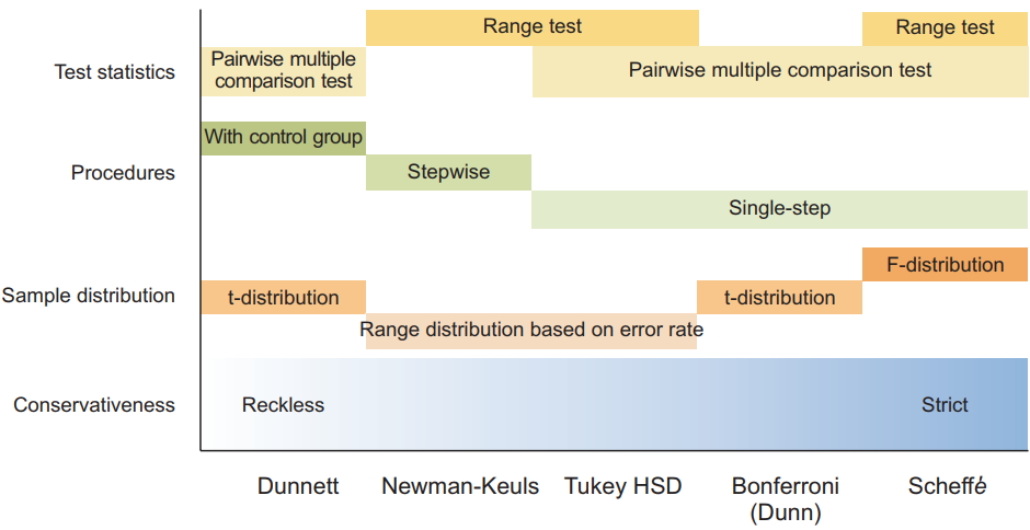
In a study, many situations occur that may affect the choice of MCTs. For example, a group might have different sample sizes. A several multiple comparison analysis tests was specifically developed to handle nonidentical groups. In the study, power can be a problem, and some tests have more power than others. Whereas all comparative tests are important in some studies, only predetermined combinations of experimental groups or comparators should be tested in others. When a special situation affects a particular pairwise analysis, the selection of multiple comparative analysis tests should be controlled by the ability of specific statistics to address the questions of interest and the types of data to be analyzed. Therefore, it is important that researchers select the tests that best suit their data, the types of information on group comparisons, and the power required for analysis (Fig. 3).
In general, most of the pairwise MCTs are based on balanced data. Therefore, when there are large differences in the number of samples, care should be taken when selecting multiple comparison procedures. LSD, Sidak, Bonferroni, and Dunnett using the t-statistic do not pose any problems, since there is no assumption that the number of samples in each group is the same. The Tukey test using the studentized range distribution can be problematic since there is a premise that all sample sizes are the same in the null hypothesis. Therefore, the Tukey-Kramer test, which uses the harmonic mean of sample numbers, can be used when the sample numbers are different. Finally, we must check whether the equilibrium of variance assumption is satisfied. The methods of multiple comparisons that have been mentioned previously are all assumed to be equally distributed. Tamhane’s T2, Dunnett’s T3, Games-Howell, and Dunnett’s C are multiple comparison tests that do not assume equilibrium.
Although the Korean Journal of Anesthesiology has not formally examined this view, it is expected that the journal’s view on this subject is not significantly different from the view expressed by this paper [8]. Therefore, it is important that all authors are aware of the problems posed by multiple comparisons, and further research is required to spread awareness regarding these problems and their solutions.