Multicollinearity and misleading statistical results
Article information

Abstract
Multicollinearity represents a high degree of linear intercorrelation between explanatory variables in a multiple regression model and leads to incorrect results of regression analyses. Diagnostic tools of multicollinearity include the variance inflation factor (VIF), condition index and condition number, and variance decomposition proportion (VDP). The multicollinearity can be expressed by the coefficient of determination
(Rh2) of a multiple regression model with one explanatory variable (Xh) as the model’s response variable and the others (Xi [i≠h] as its explanatory variables. The variance
(σh2) of the regression coefficients constituting the final regression model are proportional to the VIF
Introduction
A prospective randomized controlled trial assesses the effects of a single explanatory variable on its primary outcome variable and the unknown effects of the other explanatory variables are minimized by randomization [1]. However, in observational or retrospective studies, randomization is not performed before the collection of data and there exist the confounding effects of explanatory variables other than the one of interest. To control the confounding effects on a single response variable, multivariable regression analyses are used. However, most of the time, explanatory variables are intercorrelated and produce significant effects on one another. This relationship between explanatory variables compromises the results of multivariable regression analyses. The intercorrelation between explanatory variables is termed as “multicollinearity.” In this review, the definition of multicollinearity, measures to detect it, and its effects on the results of multiple linear regression analyses will be discussed. In the appendix following the main text, the concepts of multicollinearity and measures for its detection are described with as much detail as possible along with mathematical equations to aid readers who are unfamiliar with statistical mathematics.
Multicollinearity
Exact collinearity is a perfect linear relationship between two explanatory variables X1 and X2. In other words, exact collinearity occurs if one variable determines the other variable (e.g., X1 = 100 − 2X2). If such relationship exists between more than two explanatory variables (e.g., X1 = 100 − 2X2 + 3X3), the relationship is defined as multicollinearity. Under multicollinearity, more than one explanatory variable is determined by the others. However, collinearity or multicollinearity do not need to be exact to determine their presence. A strong relationship is enough to have significant collinearity or multicollinearity. A coefficient of determination is the proportion of the variance in a response variable predicted by the regression model built upon the explanatory variable (s). However, the coefficient of determination (R2) from a multiple linear regression model whose response and explanatory variables are one explanatory variable and the rest, respectively, can also be used to measure the extent of multicollinearity between explanatory variables. R2 = 0 represents the absence of multicollinearity between explanatory variables, while R2 = 1 represents the presence of exact multicollinearity between them. The removal of one or more explanatory variables from variables with exact multicollinearity does not cause loss of information from a multiple linear regression model.
Variance Inflation Factor
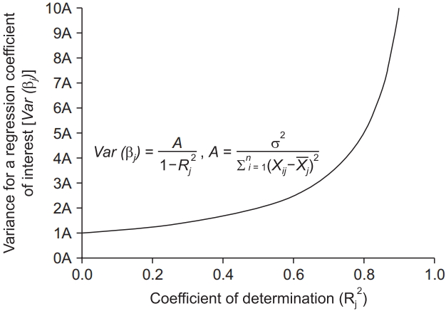
The variance of regression coefficients is proportional to
which is called the variance inflation factor. Considering the range of R2 (0 ≤ R2 ≤ 1), R2 = 0 (complete absence of multicollinearity) minimizes the variance of the regression coefficient of interest, while R2 = 1 (exact multicollinearity) makes this variance infinite (Fig. 1). The reciprocal of the variance inflation factor (1 − R2) is known as the tolerance. If the variance inflation factor and tolerance are greater than 5 to 10 and lower than 0.1 to 0.2, respectively (R2 = 0.8 to 0.9), multicollinearity exists. Although the variance inflation factor helps to determine the presence of multicollinearity, it cannot detect the explanatory variables causing the multicollinearity.
The effects of the coefficient of determination (Rj 2 ) from a regression model
As previously mentioned, strong multicollinearity increases the variance of a regression coefficient. The increase in the variance also increases the standard error of the regression coefficient (because the standard error is the square root of the variance). The increase in the standard error leads to a wide 95% confidence interval of the regression coefficient. The inflated variance also results in a reduction in the t-statistic to determine whether the regression coefficient is 0. With a low t-statistic value, the regression coefficient becomes insignificant. The wide confidence interval and insignificant regression coefficient make the final predictive regression model unreliable.
Condition Number and Condition Index
The eigenvalues (λ) obtained from the calculation using a matrix composed of standardized explanatory variables can be used to diagnose multicollinearity. The total number and sum of the eigenvalues are equal to the number of explanatory variables. The average of the eigenvalues is 1. Because the total sum of the eigenvalues is constant, the presence of their high maximum value indicates that the other eigenvalues are low relative to the maximum (λmax). Eigenvalues close to 0 indicate the presence of multicollinearity, in which explanatory variables are highly intercorrelated and even small changes in the data lead to large changes in regression coefficient estimates. The square root of the ratio between the maximum and each eigenvalue (λ1, λ2, … , λk) is referred to as the condition index:
The largest condition index is called the condition number. A condition number between 10 and 30 indicates the presence of multicollinearity and when a value is larger than 30, the multicollinearity is regarded as strong.
Variance Decomposition Proportion
Eigenvectors derived from eigenvalues are used to calculate the variance decomposition proportions, which represent the extent of variance inflation by multicollinearity and enable the determination of the variables involved in the multicollinearity. Each explanatory variable has variance decomposition proportions corresponding to each condition index. The total sum of the variance decomposition proportions for one explanatory variable is 1. If two or more variance decomposition proportions corresponding to condition indices higher than 10 to 30 exceed 80% to 90%, it is determined that multicollinearity is present between the explanatory variables corresponding to the exceeding variance decomposition proportions.
Strategies to Deal with Multicollinearity
Erroneous recording or coding of data may inadvertently cause multicollinearity. For example, the unintentional duplicative inclusion of the same variable in a regression analysis yields a multicollinear regression model. Therefore, preventing human errors in data handling is very important. Theoretically, increasing the sample size reduces the standard errors of regression coefficients and hence, decreases the degree of multicollinearity [2]. However, standard errors are not always reduced under strong multicollinearity. Old explanatory variables can be replaced with newly collected ones, which predict a response variable more accurately. However, the inclusion of new cases or explanatory variables to an already completed study requires significant additional time and cost or is simply technically impossible.
Combining multicollinear variables into one can be another option. Variables that belong to a common category are usually multicollinear. Hence, combining each variable into a higher hierarchical variable can reduce the multicollinearity. In addition, one of the variables in nearly exact collinearity can be presented by an equation with the other variable. The inclusion of the equation in the multiple regression model removes one of the collinear variables. Principal component analysis or factor analysis can also generate a single variable that combines multicollinear variables. However, with this procedure, it is not possible to assess the effect of individual multicollinear variables.
Finally, the multicollinear variables identified by the variance decomposition proportions can be discarded from the regression model, making it more statistically stable. However, the principled exclusion of multicollinear variables alone does not guarantee the remaining of the relevant variables, whose effects on the response variable should be investigated in the multivariable regression analysis. The exclusion of relevant variables produces biased regression coefficients, leading to issues more serious than multicollinearity. Ridge regression is an alternative modality to include all the multicollinear variables in a regression model [3].
Numerical Example
In this section, multicollinearity is assessed from variance inflation factors, condition numbers, condition indices, and variance decomposition proportions, using data (Table 1) from a previously published paper [4]. The response variable considered, is the liver regeneration rate two weeks after living donor liver transplantation (LDLT). Four of the six explanatory variables considered, are hepatic hemodynamic parameters measured one day after LDLT, which include the peak portal venous flow velocity (PVV), the peak systolic velocity (PSV) and the end diastolic velocity (EDV) of the hepatic artery, and the peak hepatic venous flow velocity (HVV). These parameters are standardized by dividing them by 100 g of the initial graft weight (GW). The other explanatory variables considered are the graft-to-recipient weight ratio (GRWR) and the GW to standard liver volume ratio (GW/SLV).

Because the shear stress generated by the inflow from the portal vein and hepatic artery into a partial liver graft serves as a driving force for liver regeneration [5], it is assumed that the standardized PPV, PSV, and EDV (PVV/GW, PSV/GW, and EDV/GW, respectively) are positively correlated with the liver regeneration rate. A positive correlation between the standardized HVV (HVV/GW) and liver regeneration rate is also expected because the inflow constitutes the outflow through the hepatic vein from a liver graft. In addition, the smaller is a liver graft, the higher is the shear stress. Hence, the graft weight relative to the recipient weight and standard liver volume is expected to be negatively correlated with the liver regeneration rate. The expected univariate correlations between each explanatory variable and liver regeneration rate were found in the above-cited paper [4]. Significant correlations between the hepatic hemodynamic parameters (PVV/GW, PSV/GW, EDV/GW, and HVV/GW) and between the relative graft weights (GRWR and GW/SLV) are anticipated because they share common characteristics. Therefore, the use of all of these explanatory variables for multiple linear regression analysis might lead to multicollinearity.
As expected, the correlation matrix of the explanatory variables shows a significant correlation between the variables (Table 2). Based on the regression coefficients calculated from the multiple linear regression analysis using the six explanatory variables (Table 3A), we obtain the following regression model.

Correlation Matrix between Explanatory Variables

Regression Coefficients of Multiple Linear Regression Model for Six Explanatory Variables
Liver regeneration rate = 232.797 + 0.221 × PPV ⁄ GW − 0.050 × PSV ⁄ GW + 0.690 × EDV ⁄ GW + 4.083 × HVV ⁄ GW − 0.905 × GW ⁄ SLV − 37.594 × GRWR (R2 = 0.682, P < 0.001)
While an increase in the PSV/GW leads to an increase in the liver regeneration rate, according to the results of the simple linear regression analysis [4] a unit increase in the PSV/GW reduces, albeit insignificantly, the regeneration rate by 0.05%. In addition, although the effect of a unit change in the GRWR on the regeneration rate is the strongest (37.954% decrease in the regeneration rate per unit increase), its regression coefficient is not statistically significant due to its inflated variance, which leads to a high standard error of 32.665 and a wide 95% confidence interval between –104.4 and 29.213. These unreliable results are produced by multicollinearity presented by the high variance inflation factors of the regression coefficients for GW/SLV, GRWR, and PSV/GW (more than or very close to 5), which are 7.384, 6.011, and 4.948, respectively. They are indicated with asterisks in Table 3A. The three condition indices of more than 10 (daggers in Table 3B) also indicate that there are three linear dependencies that arise from multicollinearity. However, they cannot identify the explanatory variables with multicollinearity.

Collinearity Diagnostics
The variance decomposition proportions exceeding 0.8 are indicated with asterisks in Table 3B. Those corresponding to the highest condition index (condition number), i.e., 0.99 and 0.84, indicate that the most dominant linear dependence of the regression model is explained by 99% and 84% of the variance inflation in the regression coefficients of GW/SLV and GRWR. The strong linear dependence between the two explanatory variables is also supported by the highest Pearson’s correlation coefficient (R = 0.886) between them (Table 2). However, the second strongest correlation between PSV/GW and EDV/GW (R = 0.841), which can be found in Table 2, does not seem to cause multicollinearity in the multiple linear regression model. Although the variance inflation factor of the PSV/GW (4.948) is lower than 5, it is very close to it. In addition, only one of their variance decomposition proportions corresponding to the condition index of 11.938 is over 0.8. However, if the cut-off value of the variance decomposition proportion for the diagnosis of multicollinearity is set to 0.3 according to the work of Liao et al. [6], the two explanatory variables are multicollinear. Therefore, excluding the GW/SLV from the regression model is justified, but whether the PSV/GW is removed from the regression model is not clear.
The exclusion of GW/SLV and PSV/GW produced a stable regression model (Table 4A) which is

Regression Coefficients of Multiple Linear Regression Model for Four Explanatory Variables Following the Exclusion of Two Variables
Liver regeneration rate = 209.393 + 0.392 × PVV ⁄ GW + 1.006 × EDV ⁄ GW + 4.410 × HVV ⁄ GW − 68.832 × GRWR (R2 = 0.669, P < 0.001)
All the variance inflation factors became less than 2. Particularly, the variance inflation factor of the regression coefficient for the GRWR was reduced from 6.011 to 1.137 with a decrease in its standard error from 32.665 to 14.014 and narrowing of its 95% confidence interval from (−104.4, 29.213) to (−97.413, −40.251). In accordance with the above changes, the probability value for the regression coefficient became less than 0.05 (from 0.259 to < 0.001). Although there is still a condition number of more than 10, only one variance decomposition proportion of more than 0.9 is present (Table 4B). It needs to be noted that the intercept term is not important for this analysis. The small change in the coefficient of determination (R2) from 0.682 to 0.669 indicates a negligible loss of information.

Collinearity Diagnostics
Conclusions
Multicollinearity distorts the results obtained from multiple linear regression analysis. The inflation of the variances of the regression coefficients due to multicollinearity makes the coefficients statistically insignificant and widens their confidence intervals. Multicollinearity is determined to be present if the variance inflation factor and condition number are more than 5 to 10 and 10 to 30, respectively. However, they cannot detect which explanatory variables are multicollinear. To identify the variables with multicollinearity, the variance decomposition proportion is used. If the variance decomposition proportions of more than 0.8 to 0.9 correspond to the condition indices of more than 10 to 30, the explanatory variables, which are associated with the variance decomposition proportions corresponding to common condition indices, are multicollinear. In conclusion, the diagnosis of multicollinearity and exclusion of multicollinear explanatory variables enable the formulation of a reliable multiple linear regression model.
Notes
Conflicts of Interest
No potential conflict of interest relevant to this article was reported.