Concepts and emerging issues of network meta-analysis
Article information

Abstract
Most diseases have more than two interventions or treatment methods, and the application of network meta-analysis (NMA) studies to compare and evaluate the superiority of each intervention or treatment method is increasing. Understanding the concepts and processes of systematic reviews and meta-analyses is essential to understanding NMA. As with systematic reviews and meta-analyses, NMA involves specifying the topic, searching for and selecting all related studies, and extracting data from the selected studies. To evaluate the effects of each treatment, NMA compares and analyzes three or more interventions or treatment methods using both direct and indirect evidence. There is a possibility of several biases when performing NMA. Therefore, key assumptions like similarity, transitivity, and consistency should be satisfied when performing NMA. Among these key assumptions, consistency can be evaluated and quantified by statistical tests. This review aims to introduce the concepts of NMA, analysis methods, and interpretation and presentation of the results of NMA. It also briefly introduces the emerging issues in NMA, including methods for evaluation of consistency.
Before we begin: systematic review and meta-analysis
Before the introduction of network meta-analysis (NMA), understanding the concepts and processes of systematic review and meta-analysis is necessary. A meta-analysis, including NMA, which is located higher in the hierarchy of evidence, should be preceded by and based on a systematic review [1].
In recent years, the publication of systematic reviews, meta-analyses, and network meta-analyses has increased with an increase of frequent citation [2,3]. They have become essential for making clinical decisions and developing health policies, which require balanced decisions regarding effectiveness, tasks, and resources [3]. A systematic review attempts to collate and identify the best available empirical evidence [1]. The research question of a systematic review usually focuses on pre-specified question(s). The search process for the evidence is comprehensive because a systematic review aims to find all the eligible evidence related to the research questions; it is also reproducible. The methodology for a systematic review is clear, explicit, systematic, and rigorously focused on minimizing bias, thereby providing more reliable findings [4,5]. The objective, inclusion and exclusion criteria, search strategy, selection and evaluation of articles, extraction of information, methods for data synthesis, and presentation should be determined before the commencement of the study.
However, a meta-analysis, per se, refers to a statistical analysis which quantitatively integrates and summarizes the results from separate studies [6] and investigates the source of heterogeneity [7]. A meta-analysis uses the results from multiple studies, provides more precise effect estimates, and increases statistical power [8]. Therefore, generalizing the results from individual studies aside from providing pooled analysis, a meta-analysis has the advantage of qualitatively assessing risk factors, investigating rare exposures and diseases, and studying heterogeneity (i.e., identifying the reason for the difference or dispersion between studies).
However, meta-analysis has received criticism for the following reasons: 1) a single number cannot summarize the entire research field, 2) discrepancies exist between meta-analyses and large randomized controlled trials (RCTs) [9], 3) a possible file drawer problem (publication bias) [10], and 4) mixing different kinds of studies without considering their heterogeneity causes the ‘apples and oranges’ conundrum [11]. Therefore, the validation or assessment of the quality within or between the included studies is important as it can deteriorate the validity of the meta-analysis [6].
Introduction to NMA
More than two interventions or treatment methods generally exist for most diseases, and not all existing interventions or treatment methods are directly compared. Furthermore, the continually developing interventions or treatment methods are generally compared with placebo or standard interventions or treatment methods. They are not always compared with interventions or treatments currently employed in clinical practice.
Most clinicians, patients, and health policymakers want to be aware of the interventions or treatment methods that are superior based on all available evidence. However, organizing or performing a mega-RCT that compares all existing interventions or treatment methods that analyzes their effects and harms is practically impossible.
NMA, an extension of the traditional pairwise meta-analysis, synthesizes, compares, and analyzes three or more interventions and treatment methods using both direct and indirect evidence to evaluate the effects or harms of each treatment. The NMA includes multiple groups and is also called ‘multiple-treatment meta-analysis’. Moreover, NMA includes both direct and indirect comparisons and is also called ‘mixed-treatment comparison’.
Therefore, the NMA aims to collect all the RCTs performed and to compare the effects and harms of all interventions or treatment methods. The advantages of NMA are that (1) it provides useful evidence via indirect comparison even if no previous study has directly compared the effect and harm of the interventions or treatment methods; (2) because NMA uses information from both direct and indirect evidence, it increases the precision of estimate or power compared to that when using direct evidence alone; and (3) it ranks the relative effects and harm of all interventions and treatment methods.
Direct comparison refers to comparison of two or more interventions or treatment methods within a study, whereas indirect comparison refers to comparisons of interventions or treatment methods made through one or more common comparators [12].
In Fig. 1A, the solid blue and dotted red lines indicate direct and indirect comparisons, respectively. TA, TB, TC and TD are used as abbreviated version of treatment A, B, C and D in the following manuscript and figures. In this figure, TA serves as an anchor that indirectly compares TB and TC or TB, TC, and TD. TA (anchor) is also called a common comparator. TB and TC or TC and TD are indirectly compared using anchor A. This type of comparison is called an ‘anchored indirect treatment comparison.' When the shape formed by direct comparisons is incomplete, it is also called an ‘open triangle.’
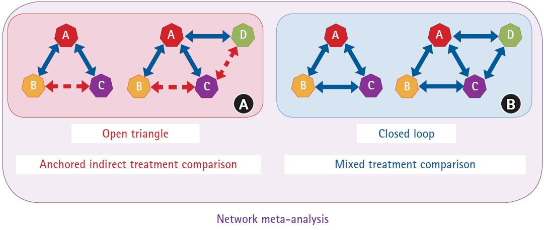
Direct and indirect comparisons in network meta-analysis. (A) Direct (TA versus TB, TA versus TC, and TA versus TD) and indirect (TB versus TC and TC versus TD) comparisons anchored by TA. Anchored indirect treatment comparison is called an open triangle. (B) Direct comparisons are called a closed loop.
A mixed-treatment comparison (Fig. 1B) exists when both direct and indirect comparisons between TB and TC and through anchor A (not shown in the figure) are noted. When the shape formed by direct comparison is complete, it is also called a ‘closed loop’. Open triangles and closed loops together, as shown in Figs. 1A and 1B, are called NMA. Mixed-treatment comparison can be explained as a generalized concept of the synthesis and summary of the effects of direct and indirect comparisons.
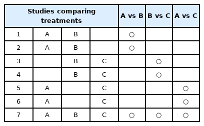
The sample NMA presented in Table 1 includes seven studies. Studies 1, 2, and 7 directly compared TA and TB; studies 5 and 6 directly compared TA and TC; and studies 3, 4, and 7 directly compared TB and TC. In addition to information from the direct comparison of TA and TB, information from the indirect comparison can also be used to compare the two treatments. TA and TB can be indirectly compared using TC as a common comparator in studies 3, 4, 5, and 6. As TC has also been investigated in study 7, TA and TB can also be indirectly compared via the common comparator TC in this study.
The Example of Studies Comparing Each Treatment
Two studies compared TA versus TB and TA versus TC (Fig. 2A). The red rectangle represents the difference between the treatment effects of TA and TB (TAB = TB − TA), and the sky blue rectangle represents the difference between the treatment effects of TA and Tc (TAC = TC – TA). The difference between the treatment effects of TB and TC (TBC) may be obtained by subtracting the treatment effect of B from that of C (TBC = TC – TB). However, it may lead to bias when the treatment effect of TA in study AB (a study that compared TA and TB is named study AB) may be different from that in study AC. Therefore, the possibility of baseline differences between studies regarding the treatment effect of A as a common comparator should be considered (Fig. 2A).

The examples to calculate treatment effects between studies. (A) TBC (difference of treatment effect between TB and TC) can be calculated as TC−TB. However, an error can occur when a difference in the treatment effect of A exists. (B) No connection between the treatments exists. TAB and TCD cannot be assumed. (C) TBC can be assumed using the common comparator TA in study AB (a study that compares TA and TB) and study AC (a study that compares TA and TC), and TAD can be assumed using the common comparator TC.
Critical views exist on indirect comparisons performed in NMA. First, although indirect comparisons assume randomization, it is not randomized evidence. All interventions or treatment methods compared are not randomized across the studies. Statistically, the indirect comparison is a specific type of meta-regression, and meta-regression only provides observational evidence. Second, constant critical voices have existed on whether indirect comparisons show better evidence compared with direct comparisons and whether NMA can be performed only by indirect comparison when no direct comparison is present [13].
Steps of NMA
Attempt to include all relevant RCTs
The first step in conducting an NMA is same as that in a conventional meta-analysis. The author should define the research question based on population, intervention, comparison, and outcome (PICO), eligibility criteria, search strategies, processes for study selection, data extraction, and quality assessment of studies. Studies that include a common comparator are important when defining the eligibility criteria.
Explore network geometry
In a scenario with studies comparing TA and TB (study AB) and TC and TD (study CD) (Fig. 2B), when no connection between the treatments is noted, the relative treatment effect between TAB (difference in the treatment effect of TA and TB) and TCD (difference in the treatment effect of TC and TD) cannot be assumed. However, with a study comparing TA and TC (study AC), TBC (difference in the treatment effect of TB and TC) can be assumed through the common comparator TA (Fig. 2C). Moreover, TAD (difference in the treatment effect of TA and TD) can be assumed through the common comparator TC (Fig. 2C).
To allow comparisons of treatment effects across all interventions and treatment methods, all included studies must be connected in the network, which means that any two treatments can be compared either directly or indirectly through a common comparator. The network plots allow visual inspection of the direct and indirect evidence (Supplementary Figs. 1A and 1B).
Assess key assumptions
NMA only provides observational evidence, as in a conventional meta-analysis, and the risk of confounding bias exists. To lower the risk of confounding bias, key NMA assumptions must be assessed. Moreover, the key assumptions, including similarity, transitivity, and inconsistency, are explained separately in the following section.
Performance of analyses and NMA
Free software, such as WinBUGS [14], R [15–17], Python, OpenBUGS [18], and ADDIS, or commercially available software, such as Stata [19], SAS, and Excel (NetMetaXL) [20], can be used to perform NMA statistics. Statistical approaches for NMA are divided into frequentist and Bayesian frameworks [12]. Frequentist NMA can be performed using R (nemeta package [21]) and Stata software [19], and Bayesian NMA can be performed using R (gemtc [16], pcnemeta [17], and BUGSnet package [15]) and WinBUGS software.
The frequentist framework NMA using Stata can be performed using the methods of White IR [19].
Key assumption in network meta-analysis
To perform NMA using data from several studies, the following three assumptions must be satisfied [22]: similarity or homogeneity assumption generally applies to direct comparisons, transitivity assumption applies to indirect comparisons, and consistency assumption applies to mixed comparisons (direct and indirect comparisons).
Similarity and homogeneity for direct comparisons
According to the concept of similarity or homogeneity, ‘combining studies should only be considered if they are clinically and methodologically similar.’ Similarity or homogeneity is observed when the true treatment effects of two interventions or treatment methods are similar in direct comparisons, and heterogeneity appears when the true treatment effect varies. Similarity should be shown in PICO; for example, the similarity assumption may be violated if the administration methods for a similar drug are different (for example, injection and oral pill). The similarity is evaluated qualitatively; therefore, testing for the statistical hypothesis is not done. Similarity or homogeneity of the methodology employed in the included studies should also be observed.
Transitivity for indirect comparisons
Transitivity is the validity for logical reasoning, which means that the difference TAB and TAC, can be used to calculate the TBC, an indirect comparison. If the treatment effect of A is similar between the direct comparison of TAB and TAC, the common comparator A can be used from TAB and TAC, which is ‘transitive’ from treatments B through A to C.
Transitivity is a conceptual definition and an assumption that cannot be calculated. However, its validity can be evaluated in terms of the clinical, epidemiological, and methodological aspects. If intransitivity is suspected, the existence of an effect modifier should be thoroughly examined.
The distribution of patient and study characteristics, which are effect modifiers, must be sufficiently similar between studies AB and AC to generalize TAB to TAC. If an imbalance in the distribution of effect modifiers exists between the studies, incorrect estimates may be obtained. Fig. 3 shows that the assumption of transitivity is violated when effect modifier D (between TA and TB) is not similar to effect modifier E (between TA and TC).
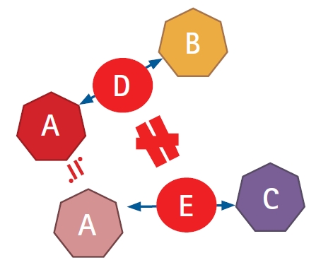
Transitivity-visualized diagram. Transitivity between studies AB and AC via TA as a common comparator. The assumption of transitivity is violated when the effect modifier D (between TA and TB) is not similar to effect modifier E (between TA and TC).
For example, if study AB included 30 male and 30 female patients and study AC included 20 male and 20 female patients, combining both would satisfy the transitivity assumption because the gender distribution is same in both studies. The assumption of transitivity is violated if an imbalance exists between studies AB and AC. However, if an imbalance exists between studies AB and AC, the transitivity assumption is assumed to be satisfied if the gender distribution does not affect the outcome (i.e., gender is not an effect modifier).
All treatments included in NMA should be ‘jointly randomizable’, which means that a trial including all treatments would be clinically reasonable. It is assumed that the investigators have included RCTs. Comparisons within an RCT are compared between the randomized groups, while those between RCTs are not randomized. However, comparisons between RCTs are not randomized. Therefore, the comparisons between RCTs should be assumed to be ‘jointly randomizable’ to perform an NMA. Thus, it is essential to consider this when conducting an evidence network. Transitivity may be violated if the intervention or treatment method has a different target patient group or indication between studies. For example, when TA is the primary treatment and TB and TC are both primary and secondary treatments, patients in study BC cannot be assumed to be randomly assigned to study AC.
Consistency for mixed comparisons
Consistency, the agreement between direct and indirect evidence for a given pair of intervention and treatment methods, is an objective assessment of transitivity during data manifestation. The consistency assumption is satisfied when the magnitude of the effect through direct and indirect comparisons is consistent. The consistency assumption is a statistical confirmation of transitivity, which can be evaluated by determining if the effect size is similar through direct and indirect comparisons. Moreover, consistency can be evaluated not in an open triangle but in a closed loop because only some comparisons are indirect in an open triangle.
Consistency is also called coherence or transitivity across loops. The four causes of inconsistencies are (1) chance, (2) genuine diversity, (3) bias in direct comparison, and (4) bias in indirect comparison [5].
Unlike similarity and transitivity, which are evaluated qualitatively, consistency is evaluated using a statistical method. Several statistical methods have been suggested to check the assumptions regarding consistency. Of these, six methods that are commonly used to assess NMA inconsistency have been described.
Cochran’s Q statistics
Cochran’s Q statistic is a commonly used method for assessing heterogeneity within the NMA [23]. When performing Cochran’s Q statistic, the null hypothesis is that the treatment effectiveness in all studies is equal. An alternative hypothesis is that the treatment effectiveness in these studies is different [24].
Cochran’s Q statistic can be calculated by summing the squared deviations of each study’s estimate from the overall meta-analytic estimate, weighting the contribution of each study. P values for Cochran’s Q statistic can be obtained using the χ2 distribution [24].
The overall Cochran’s Q statistic from the fixed-effect NMA can be used for both within- and between-design heterogeneities. However, it has lower power in detecting heterogeneity when the numbers of included studies or samples size are small.
The quantity of heterogeneity, I2, is provided to measure the degree of inconsistency. I2 can be calculated as I2 = 100% × (Q − df) / Q, where Q is Cochran’s heterogeneity statistic and df is the degree of freedom. A value of 0% indicates no heterogeneity, and larger values indicate increasing heterogeneity.
Loop inconsistency (Supplementary Fig. 2)
The Bucher method is a simple z-test developed to assess loop inconsistency in loops of three treatments with two-arm trials in a network [25]. The measurement of loop inconsistency is discussed below. The absolute value of the difference in the effect size between the direct and indirect comparisons between treatments is called the IF.
For example, IF for treatment BC is as follows:
The variance of IF, var(IF), was calculated by summing the variance of direct and indirect comparisons.
The null hypothesis is that the effect sizes of the direct and indirect comparisons are equal, and the alternative hypothesis is that the effect sizes of the direct and indirect comparisons are different.
A test for H0: IF = 0
A test for H1: IF ≠ 0
Z is calculated by dividing IF by the square root of var(IF), and the distribution of z follows a standard normal distribution.
The 95% CI of IF was calculated by the summation or subtraction of the square root of var(IF).
95% CI IF±1.96√var(IF)
If the 95% CI does not contain 0, the consistency assumption is rejected. These steps were repeated for each independent loop in the network.
This method has the advantages of simplicity, ease of application, and intuitive for loops with large inconsistencies. However, evaluating the consistency of the entire network and discriminating a particular comparison with a problem within the loop when inconsistency appears in the loop is difficult. Furthermore, multiple testing must be considered, which may be both cumbersome and time-consuming when this approach is applied to a large network wherein each treatment loop is considered one at a time [26,27].
Inconsistency parameter approach
One of the most popular models for evaluating NMA inconsistency is the inconsistency parameter approach proposed by Lu and Ades (Bayesian hierarchical model) [28]. This model is a generalization of the Bucher method and relaxes the assumption regarding consistency by including an inconsistency parameter (ωABC) in each loop wherein inconsistency could occur.
Consistency model
μBC = μAC - μAB
Inconsistency model
μBC = μAC - μAB + ωABC
where
μBC is the treatment effect of BC,
μAB is the treatment effect of AB,
μAC is the treatment effect of AC, and
ωABC is the inconsistency parameter.
These additional inconsistency parameters can be fitted as fixed or random effects. Models with and without inconsistency parameters are then compared to assess whether a network is consistent and arbitrarily chosen. An inconsistency model can be obtained by omitting the consistency assumption. If it is assumed that the inconsistency parameter (ωABC) is 0 in the inconsistency model, it can be classified as a consistency model. The distribution of the inconsistent variable is ωj~N(0,σ2).
Node-splitting (Supplementary Fig. 3)
Node-splitting is a conceptual extension of the loop inconsistencies. This method separates the evidence into direct and indirect evidence from the entire network and assesses the discrepancy between them, which is repeated for all treatment comparisons [29]. When all treatment nodes are split simultaneously, they can be considered equivalent to the inconsistent parameter approaches of Lu and Ades.
Different methods to evaluate potential differences in the relative treatment effects estimated by direct and indirect comparisons are grouped as local and global approaches [29]. The aforementioned three approaches, including Cochran’s Q statistic, the loop inconsistency approach, and the inconsistency parameter, provide a global assessment of network inconsistency. The node-splitting method was first proposed as a local approach to identify the treatment comparisons that cause inconsistencies [29].
Net heat plot (Supplementary Fig. 4)
Krahn et al. [30] proposed a net heat plot to identify inconsistencies within the NMA. They introduced a design-by-treatment interaction approach that relaxes one treatment loop to calculate the remaining inconsistency across the network. The net heat plot is used to check both inconsistencies and contributions. It is a matrix visualization that shows inconsistency as highlight hotspots [30] (Supplementary Fig. 2).
Design-by-treatment interaction approach
This method evaluates whether a network as a whole demonstrates inconsistency by employing an extension of a multivariate meta-regression that allows for different treatment effects in studies with different designs (the ‘design-by-treatment interaction approach’) [31] (Supplementary Fig. 2). This method simultaneously considers both heterogeneity and the inconsistency between different studies.
To exemplify the idea of the design-by-treatment interaction approach, consider a network of evidence constructed from an ABC three-arm trial and an ABCD four-arm trial. Both the ABC and ABCD trials are inherently consistent. However, these two studies are considered to have different designs, and design inconsistency reflects the possibility that they may provide different estimates for similar comparisons (AB, AC, and BC). In these multi-arm trials, the Lu and Ades model [14] (loop inconsistency) is not suitable.
If an inconsistency exists in the NMA, any errors in the data extraction process are first checked, following which the presence of potential effect modifiers in the inconsistent loop are then checked. Alternatively, subgroup analysis and meta-regression could be helpful in analyzing the effect of potential effect modifiers on the results. Sensitivity analysis can also be performed to exclude specific studies in which inconsistencies are present. Sometimes, the cause of the inconsistency cannot be elucidated, and serious inconsistency remains despite these step-by-step efforts. Thus, in such situations, it is inappropriate to synthesize data using NMA.
Statistical methods in NMA
Two approaches exist to conduct the NMA: the Bayesian and frequentist frameworks [21]. The frequentist framework regards the parameters that represent the characteristics of the population as fixed constants and infers them using the likelihood of the observed data. The frequentist framework calculates the probability under the assumption that the observed data repeats infinitely. The results of the frequentist framework are given as a point estimate (effect measures such as odds ratio, risk ratio, and mean difference) with a 95% CI. Therefore, the frequentist framework is unrelated to external information, and the probability that the research hypothesis is true within the current data is already specified. The frequentist method can only help decide whether to accept or reject the hypothesis based on the significance level.
The Bayesian framework expresses the degree of uncertainty using a probability model by applying the probability concept to the parameters. Moreover, the Bayesian methods rely not only on the probability distribution of all the model parameters given the observed data, but also on the prior beliefs from external information about the values of the parameters. It calculates the posterior probability, which is presented as a point estimate with a 95% credibility interval and is performed using Markov Chain Monte Carlo (MCMC) simulations, allowing the reproduction of the model several times until convergence (Supplementary Fig. 5) [21]. Unlike the frequentist method, the Bayesian method has the advantage of a straightforward way of making predictions and the possibility of incorporating different sources of uncertainty with a more flexible statistical model. Therefore, it is free from the effects of the large-sample assumption. Moreover, it can be used in NMAs involving a small number of studies. This method could be more logical and persuasive than the frequentist method.
Similar to the traditional pairwise meta-analysis, NMA can utilize fixed- or random-effect approaches. The fixed-effect approach assumes that the effect size and difference between each estimate from the included studies is attributable only to the sampling error. A random-effects approach assumes that the observed difference in the effect size considers not only sampling error but also the variation of true effect size across studies, called heterogeneity. When this concept is extended to NMA, the effect size estimates vary across studies as well as comparisons (direct and indirect). Therefore, both models were tested for each network.
Choosing a better NMA model that fits the included data is important when using the Bayesian approach. Convergence of models derived from MCMC simulations can be assessed using trace and density plots and the Gelman–Rubin–Brooks methods with a potential scale reduction factor of up to 1 (Supplementary Figs. 6 and 7). The deviance information criterion (DIC) for changes in heterogeneity and statistical methods can also be used for model fit. However, a low DIC is more suitable (Supplementary Fig. 8).
Result presentation
Network plot
The network plot is a concise visual presentation of the evidence. The network plot is composed of nodes and edges, wherein the nodes represent the interventions or treatment methods compared, and the edges represent the available direct comparison between interventions or treatment methods. In some packages or programs, the size of the nodes is proportional to the number of patients, and the widths of the edges are proportional to the amount of data (for example, the number of studies directly compared or 1/standard error of treatment effect2; Supplementary Figs. 1A and 1B).
The network plot is sometimes used to check the transitivity assumption using a weighted edge proportional to the effect modifier (for example, baseline risk) or applying color by a possible effect modifier (for example, risk of bias).
Contribution plot
The contribution plot is a diagram presenting the contribution of each direct comparison to the estimation of the network summary effect. In the contribution plot, the size of each square is proportional to the weight that is attached to each direct comparison (horizontal axis) and the estimation of each network summary effect (vertical axis). The number represents the weight percentage (Supplementary Fig. 9).
Net heat plot
The net heat plot, an extension of the contribution plot, is a diagram that checks both contribution and inconsistency. In the net heat plot, the size of each square has a similar meaning to that in the contribution plot. The net heat plot also presents a matrix visualization that shows inconsistency as highlight hotspots [31]. The color of the diagonal line indicates the contribution to design inconsistency, and the color outside the diagonal indicates the degree of inconsistency between the direct and indirect rationale of the design (Supplementary Fig. 4).
Predictive interval plot
A predictive interval plot (Supplementary Fig. 10) is a forest plot of the estimated summary effects, along with their CIs and their corresponding predictive intervals. The predictive interval shows the range of values of future results in specified settings of the predictors [32]. If a new observation is added, the 95% confidence will fall within this range.
Credible interval plot
The credible interval plot (Supplementary Fig. 11) is a forest plot of the estimated summary effects, along with their credible intervals. A credible interval is that in which an unobserved parameter value falls with a particular probability in Bayesian statistics.
League table
The league table shows the relative effectiveness of possible pairs of interventions and their 95% CI (Supplementary Fig. 12). For example, the first cell in the upper left corner shows that propofol has a postoperative nausea (PON) incidence risk ratio of 0.77 (0.02–23.96) compared with palonosetron. Further, propofol shows a PON incidence risk ratio of 0.14 (0.01–2.54) compared with dexamethasone.
Rankogram and cumulative ranking curve
The rankogram presents the probabilities of each intervention or treatment method to be ranked at a specific place (1, 2, 3, etc.), based on the results of the NMA (Supplementary Fig. 13). The cumulative ranking curve represents the cumulative probabilities to reach a corresponding rank (the sum of the probabilities from those ranked 1, 2, 3, and so on; Supplementary Fig. 14). Using a cumulative ranking curve, the treatments can be ranked according to the surface under the cumulative ranking curves (SUCRA) by summing all cumulative probabilities in the cumulative ranking curve for each intervention or treatment method. The SUCRA value represents the probability that a treatment is among the best options. The Y-axis of the SUCRA value indicates the certainty of effectiveness in the network. Therefore, the rank of an intervention in the network is higher if the intervention has a larger SUCRA value (Supplementary Fig. 15).
Emerging issues of network meta-analysis
Multicomponent intervention and treatment method
In standard NMA, all existing intervention and treatment methods are considered different nodes. However, an alternative model that utilizes the information that some intervention and treatment methods are combinations of common components is called component network meta-analysis (CNMA) [33]. Let us consider a network of six treatments presented in Fig. 4 that includes three two-arm studies comparing treatments A with B + C, B with A + C, and A + B with C. If no subnetwork is connected to the others, the networks are illustrated in Fig. 4A, which shows disconnected networks. CNMA models allow ‘reconnecting’ a disconnected network if the treatment and intervention methods have common components. Fig. 4B shows that all studies have common components A, B, and C, and their contributions can be estimated using the CNMA model. CNMA has two models (additive and interactive). The additive CNMA model assumes that a combination of A and B (A + B) has similar treatment effects with the sum of treatment effects A and B. The interactive CNMA model allows for the interaction between treatments A and B. These models can now be analyzed in a frequentist framework using the R package netmeta.

Network of six treatments that includes three two-arm studies comparing treatments A with B + C, B with A + C, and A + B with C. (A) A disconnected network of three two-arm studies with six treatments. (B) The component network meta-analysis (CNMA) model enables connections between the treatments having common components.
Multiple outcome-borrowing information
For multiple outcome settings, the standard NMA model can be extended by borrowing information across outcomes as well as across studies by modeling the within- and between-study correlation structure. For the next stage, the additional assumption that intervention effects are exchangeable between outcomes is utilized to predict effect estimates for all outcomes. Moreover, multivariate meta-analysis has more areas of meta-analysis to compare treatments with two or more endpoints [34,35]. The multivariate approach has an advantage over the univariate approach because it accounts for the interrelationship between outcome and borrowed strength across studies and across outcomes via the modeling of the correlation structure [36]. NMA is another rapid methodological development area [37], and multiple outcome settings extended by borrowing information have been proposed to enhance NMA methodology [38,39].
Conclusion
NMA is a meta-analysis that synthesizes, compares, and analyzes three or more intervention/treatment methods, including both direct and indirect evidence extracted from various studies. Moreover, NMA collects information from direct and indirect evidence, which improves estimate precision. Furthermore, NMA can compare the relative effects and rank the effects of all interventions of treatments. Although indirect comparison assumes randomization, this does not mean that randomization has been performed. Therefore, assumptions of similarity, transitivity, and consistency must be satisfied for NMA; there are various strategies to overcome this challenge, and an NMA should not be performed unless these criteria are satisfied.
Notes
Conflicts of Interest
No potential conflict of interest relevant to this article was reported.
Author Contributions
EunJin Ahn (Investigation; Methodology; Project administration; Validation; Visualization; Writing – original draft; Writing – review & editing)
Hyun Kang (Conceptualization; Data curation; Formal analysis; Funding acquisition; Investigation; Methodology; Project administration; Resources; Software; Supervision; Validation; Visualization; Writing – original draft; Writing – review & editing)
Supplementary Materials
Network plot. (A) The nodes indicate the type of intervention or treatment method, and edges indicate direct comparison between intervention or treatment method. The size of nodes is proportional to the number of patients included and the width of the edges is proportional to the amount of information available (1⁄standard error of treatment effect2). This figure is produced using STATA software. (B) The nodes indicate the type of intervention or treatment method, and edges indicate direct comparison between intervention or treatment method. The size of nodes is proportional to the number of patients included and the width of the edges is proportional to the amount of information available (number of studies directly compared). This figure is produced using R software (netmeta package).
Loop inconsistency. This plot evaluates the inconsistency of the network using a design-by-treatment interaction model in multi-arm trials. Dot and black line indicate the mean and 95% confidence interval of loop inconsistency. When 95% confidence interval includes “0”, the assumption of consistency is satisfied. However, 95% confidence interval does not include “0”, the assumption of consistency is satisfied.
Node-splitting plot. The forest plot shows a difference between the direct and indirect evidence for each pairwise comparison after node-splitting. White circle and black line indicate the mean and 95% confidence interval of loop inconsistency. This method is a conceptual extension of loop inconsistency. Node-splitting methods separates the evidence into the direct and indirect evidence from entire network and assessing the discrepancy between them, and repeated for all treatment comparisons.
Net heat plot. The gray square indicates the degree to which treatment located in the column contributes to the overall estimate of the row. The color of the diagonal line means the contribution to the inconsistency of the design, and the color outside the diagonal means the degree of inconsistency between the direct/indirect rationale of the design.
Markov chain Monte Carlo (MCMC) flow chart. Markov chain Monte Carlo (MCMC) simulation and convergence diagnosis. Flow char of network meta-analysis using the “gemtc” R package using the Bayesian method. MCMC, Markov chain Monte Carlo; DIC, deviance information criterion. The process is follows as below. After coding the data, setup the network. After setting the network, select network model (fixed or random). To verify if the MCMC simulation converged well, you can check MCMC error, DIC (deviance information criterion), trace plot, density plot and Gelman-Rubin statistics. Then, select the MCMC convergence optimal model. Inconsistency test, forest plot, treatment ranking, league table can be performed.
Trace and density plot. A trace plot shows the values that the relevant parameter took during the runtime of the chain, and density plot is the histogram of the values in the trace-plot of the relevant parameter in the chain. The trace plot with no specific pattern and with entangled chains, the convergence can be considered to be good. The density plot with significant difference for the same number of simulation means the convergence is not good.
Gelman-Rubin-Brooks Plot. In Gelman-Rubin-Brooks methods, as potential scale reduction factor (PSRF) approaches 1, and the variations must be stabilized as the number of simulations increases. When PSRF approached to 1, and stabilized, it means good convergence.
Bayesian Statistics. DIC (deviance information criterion). DIC=Dbar+pD. The deviance information criterion (DIC) is expressed as DIC=Dbar+pD, where Dbar is the sum of residual deviances and pD is an estimated value of the parameter. Thus, the DIC considers both the fitness and complexity of the model, and the smaller the DIC is, the better the model.
Contribution plot. The size of each square is proportional to the weight which is attached to each direct comparison (horizontal axis) to the estimation each network summary effect (vertical axis). The number presents the weight as percentage.
Predictive interval plot. Forest plot of success rate of supraglottic airway devices. Prl: predictive intervals. Black line represents 95% confidence interval. Red line represents 95% predictive interval. I-gel versus FLMA shows significant result when presented by 95% confidence interval. However, considering 95% predictive interval, which shows the range of values of the future result, the result become insignificant.
Credible interval plot. Forest plot showing credible interval. Crl: credible intervals. Black outline circle represents odds ratio, and black line represents 95% credible interval. Credible interval is an interval within which an unobserved parameter value falls with a particular probability in Bayesian statistics.
League table. RR (95% CI) is calculated between both horizontal axis treatment and vertical axis treatment. Comparisons between treatments should be read from left to right, and the estimates in the cell in common between the vertical axis treatment and the horizontal axis treatment. Treatments are reported from left upper quadrant to right lower quadrant as per the cluster ranking for transition and acceptability. For transition, an RR less than 1 favors the row-defined treatment. For acceptability, an RR less than 1 favors the row-defined treatment. RR: relative ration; CI: confidence interval.
Rankogram. Profiles indicate the probabilities for treatments to assume any of the possible ranks. It is the probability that a given treatment ranks first, second, third, and so on, among all of the treatments evaluated in the NMA.
The cumulative ranking curves. The profile indicates the sum of the probabilities from those ranked first, second, third, and so on. A higher cumulative ranking curve (surface of under cumulative ranking curve [SUCRA]) value is regarded as an improved result for an individual’s intervention. When ranking treatments, the closer the SUCRA value is to 100%, the higher the treatment ranking is relative to all other treatments.
SUCRA-Mean Ranking. Each color represents a group of treatment that belong to the same cluster. Treatments represented in the right upper quadrant are more effective and acceptable compare to the left lower quadrant.