


Introduction
The differences in the means of two groups that are mutually independent and satisfy both the normality and equal variance assumptions can be obtained by comparing them using a Student's t-test. However, we may have to determine whether differences exist in the means of 3 or more groups. Most readers are already aware of the fact that the most common analytical method for this is the one-way analysis of variance (ANOVA). The present article aims to examine the necessity of using a one-way ANOVA instead of simply repeating the comparisons using Student's t-test. ANOVA literally means analysis of variance, and the present article aims to use a conceptual illustration to explain how the difference in means can be explained by comparing the variances rather by the means themselves.
Significance Level Inflation
In the comparison of the means of three groups that are mutually independent and satisfy the normality and equal variance assumptions, when each group is paired with another to attempt three paired comparisons1), the increase in Type I error becomes a common occurrence. In other words, even though the null hypothesis is true, the probability of rejecting it increases, whereby the probability of concluding that the alternative hypothesis (research hypothesis) has significance increases, despite the fact that it has no significance.
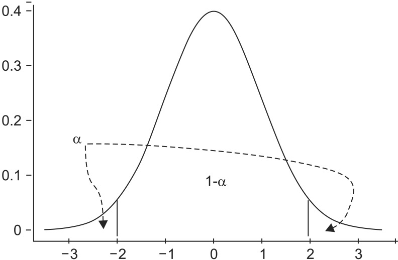
Let us assume that the distribution of differences in the means of two groups is as shown in Fig. 1. The maximum allowable error range that can claim ŌĆ£differences in means existŌĆØ can be defined as the significance level (╬▒). This is the maximum probability of Type I error that can reject the null hypothesis of ŌĆ£differences in means do not existŌĆØ in the comparison between two mutually independent groups obtained from one experiment. When the null hypothesis is true, the probability of accepting it becomes 1-╬▒.
Now, let us compare the means of three groups. Often, the null hypothesis in the comparison of three groups would be ŌĆ£the population means of three groups are all the same,ŌĆØ however, the alternative hypothesis is not ŌĆ£the population means of three groups are all different,ŌĆØ but rather, it is ŌĆ£at least one of the population means of three groups is different.ŌĆØ In other words, the null hypothesis (H0) and the alternative hypothesis (H1) are as follows:
Therefore, among the three groups, if the means of any two groups are different from each other, the null hypothesis can be rejected.
In that case, let us examine whether the probability of rejecting the entire null hypothesis remains consistent, when two continuous comparisons are made on hypotheses that are not mutually independent. When the null hypothesis is true, if the null hypothesis is rejected from a single comparison, then the entire null hypothesis can be rejected. Accordingly, the probability of rejecting the entire null hypothesis from two comparisons can be derived by firstly calculating the probability of accepting the null hypothesis from two comparisons, and then subtracting that value from 1. Therefore, the probability of rejecting the entire null hypothesis from two comparisons is as follows:
If the comparisons are made n times, the probability of rejecting the entire null hypothesis can be expressed as follows:
It can be seen that as the number of comparisons increases, the probability of rejecting the entire null hypothesis also increases. Assuming the significance level for a single comparison to be 0.05, the increases in the probability of rejecting the entire null hypothesis according to the number of comparisons are shown in Table 1.
ANOVA Table
Although various methods have been used to avoid the hypothesis testing error due to significance level inflation, such as adjusting the significance level by the number of comparisons, the ideal method for resolving this problem as a single statistic is the use of ANOVA. ANOVA is an acronym for analysis of variance, and as the name itself implies, it is variance analysis. Let us examine the reason why the differences in means can be explained by analyzing the variances, despite the fact that the core of the problem that we want to figure out lies with the comparisons of means.
For example, let us examine whether there are differences in the height of students according to their grades (Table 2). First, let us examine the ANOVA table (Table 3) that is commonly obtained as a product of ANOVA. In Table 3, the significance is ultimately determined using a significance probability value (P value), and in order to obtain this value, the statistic and its position in the distribution to which it belongs, must be known. In other words, there has to be a distribution that serves as the reference and that distribution is called F distribution. This F comes from the name of the statistician Ronald Fisher. The ANOVA test is also referred to as the F test, and F distribution is a distribution formed by the variance ratios. Accordingly, F statistic is expressed as a variance ratio, as shown below.
Here, ╚▓i is the mean of the group i; ni is the number of observations of the group i; ╚▓ is the overall mean; K is the number of groups; Yij is the jth observational value of group i; and N is the number of all observational values.
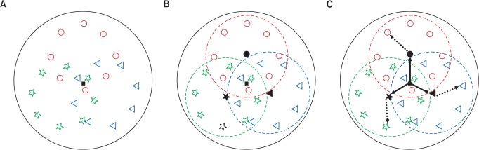
It is not easy to look at this complex equation and understand ANOVA at a single glance. The meaning of this equation will be explained as an illustration for easier understanding. Statistics can be regarded as a study field that attempts to express data which are difficult to understand with an easy and simple ways so that they can be represented in a brief and simple forms. What that means is, instead of independently observing the groups of scattered points, as shown in Fig. 2A, the explanation could be given with the points lumped together as a single representative value. Values that are commonly referred to as the mean, median, and mode can be used as the representative value. Here, let us assume that the black rectangle in the middle represents the overall mean. However, a closer look shows that the points inside the circle have different shapes and the points with the same shape appear to be gathered together. Therefore, explaining all the points with just the overall mean would be inappropriate, and the points would be divided into groups in such a way that the same shapes belong to the same group. Although it is more cumbersome than explaining the entire population with just the overall mean, it is more reasonable to first form groups of points with the same shape and establish the mean for each group, and then explain the population with the three means. Therefore, as shown in Fig. 2B, the groups were divided into three and the mean was established in the center of each group in an effort to explain the entire population with these three points. Now the question arises as to how can one evaluate whether there are differences in explaining with the representative value of the three groups (e.g.; mean) versus explaining with lumping them together as a single overall mean.
First, let us measure the distance between the overall mean and the mean of each group, and the distance from the mean of each group to each data within that group. The distance between the overall mean and the mean of each group was expressed as a solid arrow line (Fig. 2C). This distance is expressed as (╚▓i ŌłÆ ╚▓)2, which appears in the denominator of the equation for calculating the F statistic. Here, the number of data in each group are multiplied, ni(╚▓i ŌłÆ ╚▓)2. This is because explaining with the representative value of a single group is the same as considering that all the data in that group are accumulated at the representative value. Therefore, the amount of variance which is induced by explaining with the points divided into groups can be seen, as compared to explaining with the overall mean, and this explains inter-group variance.
Let us return to the equation for deriving the F statistic. The meaning of (Yij ŌłÆ ╚▓i)2 in the numerator is represented as an illustration in Fig. 2C, and the distance from the mean of each group to each data is shown by the dotted line arrows. In the figure, this distance represents the distance from the mean within the group to the data within that group, which explains the intragroup variance.
By looking at the equation for F statistic, it can be seen that this inter- or intragroup variance was divided into inter- and intragroup freedom. Let us assume that when all the fingers are stretched out, the mean value of the finger length is represented by the index finger. If the differences in finger lengths are compared to find the variance, then it can be seen that although there are 5 fingers, the number of gaps between the fingers is 4. To derive the mean variance, the intergroup variance was divided by freedom of 2, while the intragroup variance was divided by the freedom of 87, which was the overall number obtained by subtracting 1 from each group.
What can be understood by deriving the variance can be described in this manner. In Figs. 3A and 3B, the explanations are given with two different examples. Although the data were divided into three groups, there may be cases in which the intragroup variance is too big (Fig. 3A), so it appears that nothing is gained by dividing into three groups, since the boundaries become ambiguous and the group mean is not far from the overall mean. It seems that it would have been more efficient to explain the entire population with the overall mean. Alternatively, when the intergroup variance is relatively larger than the intragroup variance, in other word, when the distance from the overall mean to the mean of each group is far (Fig. 3B), the boundaries between the groups become more clear, and explaining by dividing into three group appears more logical than lumping together as the overall mean.
Ultimately, the positions of statistic derived in this manner from the inter- and intragroup variance ratios can be identified from the F distribution (Fig. 4). When the statistic 3.629 in the ANOVA table is positioned more to the right than 3.101, which is a value corresponding to the significance level of 0.05 in the F distribution with freedoms of 2 and 87, meaning bigger than 3.101, the null hypothesis can be rejected.
Post-hoc Test
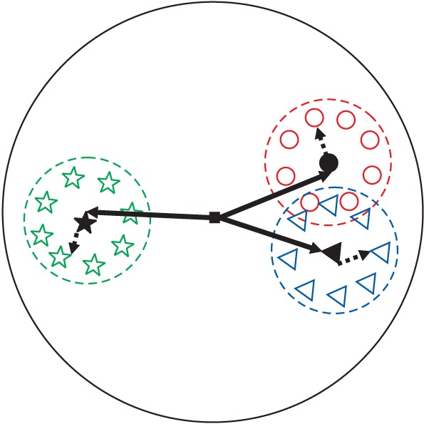
Anyone who has performed ANOVA has heard of the term post-hoc test. It refers to ŌĆ£the analysis after the factŌĆØ and it is derived from the Latin word for ŌĆ£after that.ŌĆØ The reason for performing a post-hoc test is that the conclusions that can be derived from the ANOVA test have limitations. In other words, when the null hypothesis that says the population means of three mutually independent groups are the same is rejected, the information that can be obtained is not that the three groups are different from each other. It only provides information that the means of the three groups may differ and at least one group may show a difference. This means that it does not provide information on which group differs from which other group (Fig. 5). As a result, the comparisons are made with different pairings of groups, undergoing an additional process of verifying which group differs from which other group. This process is referred to as the post-hoc test.
The significance level is adjusted by various methods [1], such as dividing the significance level by the number of comparisons made. Depending on the adjustment method, various post-hoc tests can be conducted. Whichever method is used, there would be no major problems, as long as that method is clearly described. One of the most well-known methods is the Bonferroni's correction. To explain this briefly, the significance level is divided by the number of comparisons and applied to the comparisons of each group. For example, when comparing the population means of three mutually independent groups A, B, and C, if the significance level is 0.05, then the significance level used for comparisons of groups A and B, groups A and C, and groups B and C would be 0.05/3 = 0.017. Other methods include Turkey, Sch├®ffe, and Holm methods, all of which are applicable only when the equal variance assumption is satisfied; however, when this assumption is not satisfied, then Games Howell method can be applied. These post-hoc tests could produce different results, and therefore, it would be good to prepare at least 3 post-hoc tests prior to carrying out the actual study. Among the different types of post-hoc tests it is recommended that results which appear the most frequent should be used to interpret the differences in the population means.
Conclusions
It is believed that a wide variety of approaches and explanatory methods are available for explaining ANOVA. However, illustrations in this manuscript were presented as a tool for providing an understanding to those who are dealing with statistics for the first time. As the author who reproduced ANOVA is a non-statistician, there may be some errors in the illustrations. However, it should be sufficient for understanding ANOVA at a single glance and grasping its basic concept.
ANOVA also falls under the category of parametric analysis methods which perform the analysis after defining the distribution of the recruitment population in advance. Therefore, normality, independence, and equal variance of the samples must be satisfied for ANOVA. The processes of verification on whether the samples were extracted independently from each other, Levene's test for determining whether homogeneity of variance was satisfied, and Shapiro-Wilk or Kolmogorov test for determining whether normality was satisfied must be conducted prior to deriving the results [2,3,4].