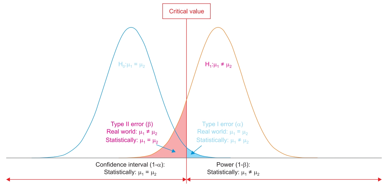
Science is based on probability. It is impossible to say with certainty whether the events observed in nature will occur or not. The same rule applies when testing hypotheses through research. Null hypotheses are basically assumed to be true. Fig. 1 presents two normal distribution probability density curves under the respective assumptions that the null hypothesis is true (left) or false (alternative hypothesis is true, right). They show the typical curves that approach but never reach the x-axis on both ends. Whether the assumption is true or not, the probability never becomes zero; this means that any result obtained from research always has a possibility of unreliability. It is always possible for conclusions from research to be wrong, and an appropriate hypothesis is required to conduct research as well as to reduce the risk of false conclusions.

If the null hypothesis is concluded to be true when the value is less than a specific point on the x-axis, and false when the value is greater, then the point is called the critical value. The probability curve of the null hypothesis partially exists on the right side of the critical value. This means that the null hypothesis is true, but as it exceeds the critical value, it is mistakenly thought to be false; this is called a Type I error. In contrast, even if the null hypothesis is false (orange probability distribution curve), because it exceeds the critical value, it is mistakenly accepted to be true; this is called a Type II error. The size of the error can be represented with a probability, which is the area under the curve lying outside the critical value. The probability of a Type I error is called the α or level of significance. The probability of a Type II error is called β. Subtracting α from the probability of the null hypothesis becomes the confidence interval, and subtracting β from the probability of the alternative hypothesis becomes the power. Under the assumption that the null hypothesis is true, the P value—the probability of observing the test statistic of the data—can be obtained. In order to determine whether the hypothesis is true or false, it is necessary to confirm whether the observed event is statistically likely to occur under the assumption that the hypothesis is true. The P value is compared to a preset standard that determines the null hypothesis as false, which is the α. The α is the standard which has been agreed upon by researchers seeking the unknown truth, but the truth cannot be certain even if the P value is less than the α. The conclusion drawn from data analysis may not be the truth, and this is the error previously mentioned. Type I and Type II errors occur once we set a critical value; they show a pattern of trade-off between α and β, the probabilities of error. As can be seen in Fig. 1, the power means the probability of rejecting the null hypothesis when the alternative hypothesis is true; the power increases as the sample size increases.

The same rule applies to the normality test. The conditions required to conduct a t-test include the measured values in ratio scale or interval scale, simple random extraction, homogeneity of variance, appropriate sample size, and normal distribution of data. The normality assumption means that the collected data follows a normal distribution, which is essential for parametric assumption. Most statistical programs basically support the normality test, but the results only include P values and not the power of the normality test. Is it possible to conclude that the data follows a normal distribution if the P value is greater than or equal to α in the normality test? This article starts from this question and discusses the relationships between the sample size, normality, and power.

Statistical analysis methods based on acquired data are divided into parametric methods and nonparametric methods, according to the normality of the data. When the data satisfies the normality, it shows a probability distribution curve with the highest frequency of occurrence at the center, and the frequency decreases with distance from the center. The distance from the center of the curve makes it easier to statistically determine whether the data obtained is frequently observed. Since most of the data are gathered around the mean value, it reflects the nature of the group and gives information on whether there is a difference between groups and the magnitude of the difference. On the other hand, if the data does not follow the normal distribution, there is no guarantee that it is centered on the mean. Therefore, the comparison of characteristics between groups using the mean value is not possible. In this case, the nonparametric test is used, in which the observations are ranked or signed (e.g., + or −), and the sums are compared. However, the nonparametric test is somewhat less powerful than the parametric test [1]. Moreover, it is only possible to detect the difference between the values of groups but not to compare the magnitude of these differences. Therefore, it is recommended that statistical analysis be performed using the parametric test if possible [1], and that the normality of the data be the first thing confirmed by the parametric test. The hypothesis in normality testing is as follows:

H₀: The data follows a normal distribution.

H₁: The data does not follow a normal distribution.

Thus, how many samples would be appropriate to assume normal distribution and to perform parametric tests?

According to the central limit theorem, the distribution of sample mean values tends to follow the normal distribution regardless of the population distribution if the sample size is large enough [2]. For this reason, there are some books which suggest that if the sample size per group is large enough, the t-test can be applied without the normality test. Strictly speaking, this is not true. Although the central limit theorem guarantees the normal distribution of the sample mean values, it does not guarantee the normal distribution of samples in the population. The purpose of the t-test is to compare certain characteristics representing groups, and the mean values become representative when the population has a normal distribution. This is the reason why satisfaction of the normality assumption is essential in the t-test. Therefore, even if the sample size is sufficient, it is recommended that the results of the normality test be checked first. Wellknown methods of normality testing include the Shapiro–Wilks test and the Kolmogorov–Smirnov test. Hence, can the t-test be conducted with a very small sample size (e.g., 3) if the normality test is satisfied?

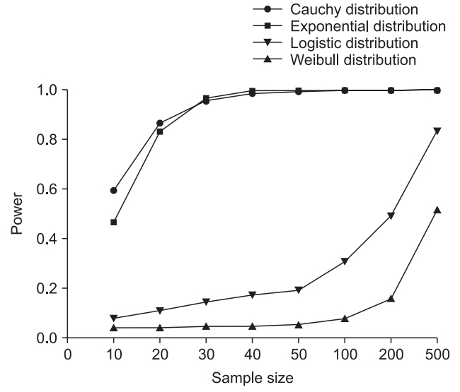
In the Shapiro–Wilks test, which is known as one of the most powerful normality tests, it is theoretically possible to perform the normality test with three samples [3,4]. However, even if the P value is greater than the significance level of 0.05, this does not automatically mean that the data follows a normal distribution. Type I and Type II errors occur in all hypothesis tests, which are detected using the significance levels and power. In general, statistical programs provide only a P value for the Type I error as a result of normality testing, and do not provide power for the Type II error. The power of the normality test indicates the ability to discriminate non-normal distributions from normal distributions. Since there is no formula that can calculate the power of the normality test directly, it is estimated by computer simulation. In the simulation, the computer repeatedly extracts samples of a certain size from the distribution to be tested, and tests whether the extracted samples have a normal distribution at a determined significance level. The power is the rate at which the null hypothesis is rejected from the data obtained through simulations repeated over several hundred times. If there are only three samples, it may be difficult to ensure that these are not normally distributed. Khan and Ahmad [4] reported the change of power according to sample sizes under different alternate non-normal distributions (Fig. 2). In fact, the types of distributions mentioned in the figure are not commonly observed in clinical studies, and are not essential to understand this figure. We do not explained in detail about that becauseit goes beyond our scope. The x-axis represents the number of samples extracted from each distribution type, and the y-axis represents the power of the normality test corresponding to the number of extracted samples. Fig. 2 shows that, although there are some degree of difference depending on the patterns of distribution, the power tends to decrease when the sample size decreases even if the significance level is fixed at 0.05. Therefore, in typical circumstances where the distribution pattern of the population is unknown, the normality test should be conducted with a sufficient sample size.

When designing a study using the t-test, it is ideal to have the same sample size for the experimental and control groups [5]. However, as in cases of studying the therapeutic effects of drugs on rare diseases, there are cases in which it is difficult to secure enough samples for the experimental group. It is well understood that increasing the sample size is a good way to improve both the significance level and the power. If so, would it be effective to increase only the sample size of control group without increasing that of the experimental group?

Assume that both sample groups follow the normal distribution and the variances are homogeneous. Assuming that sample group 1 is the experimental group and sample group 2 is the control group, the t- statistic can be expressed as [6]

where X1¯ and X2¯ are the mean values of sample groups 1 and 2, n₁ and n₂ are the sample sizes of sample groups 1 and 2, and S₍₁₊₂₎ is the pooled standard deviation of the two sample groups. Assume that t₁ is a t-statistic when the sample sizes of the two groups are the same (n₁=n₂), and t₂ is a t-statistic when the sample size of the control group is two times larger than that of the experimental group (2n₁=n₂). In the equation, n₂ can be replaced by n₁ and summarized as follows:

The above two equations can be concatenated so that t₂ can be expressed as a relation with t₁ as follows:

When the sample size of the control group is doubled, the t-statistic increases by 23 times compared with the t-statistic when the sample size is not changed. This change results in the decrease of the P value. Therefore, if it is difficult to increase the sample size of the experimental group, it can be helpful to increase the sample size of the control group instead to improve the results. However, in such cases, relatively larger sample sizes are needed to obtain similar statistical results.

Table 1 shows the results of the minimum sample size calculation required to obtain a statistically significant result in the two-tailed independent t-test at a significance level of 0.05 and power of 0.8, when the ratios of sample sizes between groups are 1 : 1 and 1 : 2, respectively. Increasing the sample size of the control group can also reduce the size of the experimental group required to achieve the same statistical result. However, instead of reducing the sample size of the experimental group by 25%, the size of the control group should be increased by 50%, which involves additional effort, time, and cost. Power becomes maximum when the sample sizes of the two groups are the same. When the variances of the two groups to be compared are similar, the smallest sample size is acquired when those of the two groups are the same [5]. Table 2 shows the change of power in two-tailed independent t-tests under the same sample size but different sample size ratios. These results suggest that increasing the sample size of the control group cannot be used as a shortcut and should only be considered in unavoidable circumstances.

It should be noted that, when the sample size ratios between groups is different, more attention should be paid to the homogeneity of variance, one of the basic assumptions of the t-test. Clinical studies generally have small sample sizes. The smaller the sample size, the greater the influence of the values of individual samples on variance. This variability becomes stable as the sample size increases. If the sample sizes of the groups are different, then this difference in variability may result in different variances.

Thus far, we have dealt with questions related to the basic assumptions of the t-test that can be found in the research design process. In the normality test, if the sample size is small, the power is not guaranteed. Therefore, it is necessary to secure a sufficient sample size. In order to maximize the power in the t-test, it is most efficient to increase the sample size of both groups equally. The above information may not be necessary for a researcher who has a sufficient sample size and conducts formal research. However, a deep understanding of the basic assumptions of the t-test will help you to understand a higher-level statistical analysis method. This will help you to take a leading role in the research process from research design to the statistical analysis and interpretation of results.